Informed Search

Informed search is an approach to solving problems with a start state to a goal state, that is based on some mathematical concepts that estimate our distance to a goal state and inform us about some of following states.

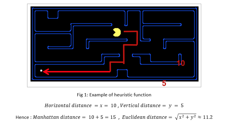
This approach needs a function called “Heuristic”, that estimates the distance to the goal state from the current state, so that it can help us find an optimal way (way with the least cost) to reach the goal. This function can be considered based on different points of view and logical explanation of the approximal distance to goal state in the problem. Such as the following example that we can consider the heuristic function based on two points of view (Euclidean distance and Manhattan distance).

Greedy Search

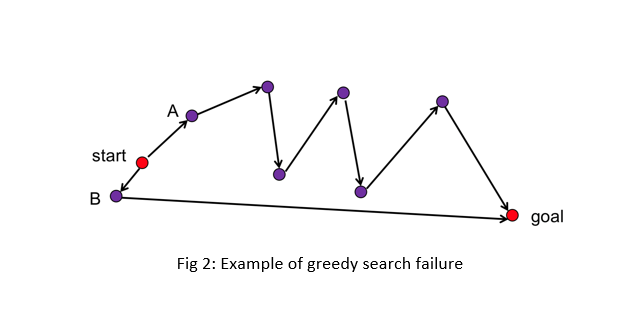
Greedy search is an approach for finding the best way to goal state considering that in each step we choose the state that is the nearest state to goal state. Therefore in such problem it is so important that the heuristic function be exact to an acceptable extent so that the estimation of distance from goal do not end in any wrong decisions. For instance, the following figure shows a situation that our heuristic (Manhattan and Euclidean distance) with faces trouble in finding the best route to goal. The best route is through B to goal, but the greedy search with the heuristic chooses the route to goal that passes through A.

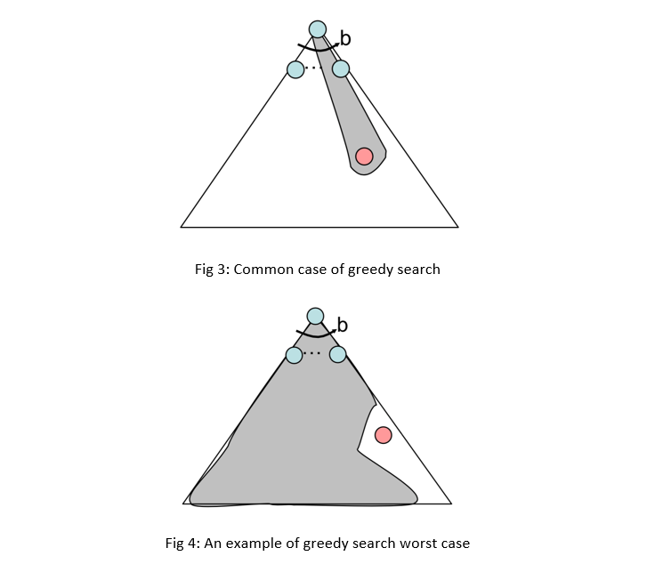
In common cases greedy search can lead to an optimal (or a suboptimal) goal as shown in fig 3. But in worst case (like badly-guided DFS) can explore every state except the goal state or can end in loops if cycle check is not considered , therefore greedy search is not complete generally. But in cases with finite states or cycle checks it is complete.

Greedy search does not necessarily end in best way to goal (as mentioned above) , so it is not an optimal search.

Suppose that in a greedy search , with the maximum branching factor is b and the depth of search tree is m , in each step maximumly b states get expanded and the best state with the least heuristic is selected to get expanded into maximumly b following states. This process repeats m times (depth of search tree) so the time complexity and Space complexity of the search would be O(b^m) at the most- all nodes are kept in memory. But good heuristic can dramatically improve the time and memory complexity.

A* Search

A* search was introduced by Hart ,Nilsson , and Rafael in 1968. This search is based on both sum of costs from start to a state n g(n) ,and the heuristic function of a state n to goal state h(n) ( therefor h(goal)=0). The idea is that in each step we select the state with the least value of f(n)=g(n)+h(n).

Suppose the problem is to find the best route from Arad to Bucharest. In fig 5 the map and the distance between cities are shown. In fig 6 the search tree is shown, bellow each node f(n)=g(n)+h(n) is written. You can see that how the A* search lead to the best route.

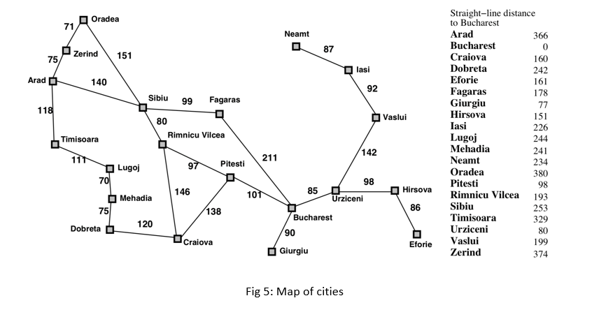
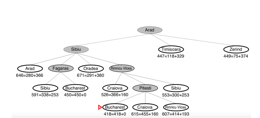
Fig 6: A*search tree of best route from Arad to Bucharest

For following topics , first we need to define two characteristics for a heuristic function h : Admissibility and Monotonicity

1) Admissibility:

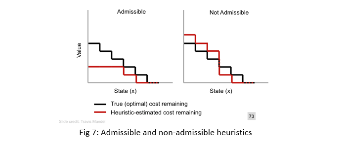
a heuristic function h is admissible if for evey node n in search tree, h(n) is less than the optimal value remaining. In fig 7 we see the difference between an admissible and a non-admissible heuristic function.

2) Monotonicity:

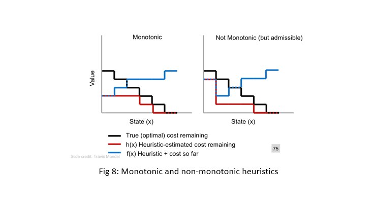
a heuristic function h is monotonic if for evey node n in search tree, f(n)=g(n)+h(n) be additive while we find the best way from start node to goal node. In fig 8 we see the difference between a monotonic and a non-monotonic heuristic function.

There are two types of A* search:

Tree-search: Repetitious states (nodes) are allowed to be inserted in the search tree
    
Graph-search: Repetitious states (nodes) are not allowed to be inserted in the search tree
    

In both cases, for reaching an optimal goal, some conditions need to be true. Theorem 1: If h(n) is admissible then A* is optimal in tree search.

Proof:

Suppose some suboptimal goal G_2 has been generated and is in the frontier. Let n be an unexpanded node in the frontier such that n is on a shortest path to an optimal goal G.

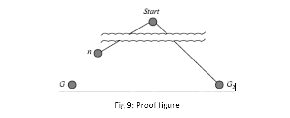
• f(G_2 )=g(G_2) since h(G_2)=0

• g(G_2)>g(G) since G_2 is suboptimal

• f(G)=g(G) since h(G)=0

• f(G_2)>f(G) from above

• h(n)≤h^* (n) (since h is admissible) hence g(n)+h(n)≤g(n)+h^* (n)

• f(n)≤g(n)+h^* (n)<f(G)<f(G_2) Hence f(G_2)>f(n), and A* will never select G_2 for expansion.

Theorem 2: If h(n) is admissible and monotonic then A* is optimal in graph search.

Proof:

A*(admissible/monotonic) will expand only nodes whose f-values are less (or equal) to the optimal cost path C* (f(n) is less-or-equal C*). 
The evaluation function of a goal node along an optimal path equals C*.

Alternative definition of monotonicity(consistency):

previously it was concluded that if in a given search path we went from state a to b and said search path was in fact monotonic then F(a)<=F(b) now based on this knowledge we are going to form another definition for monotonicity please look at the slide below:

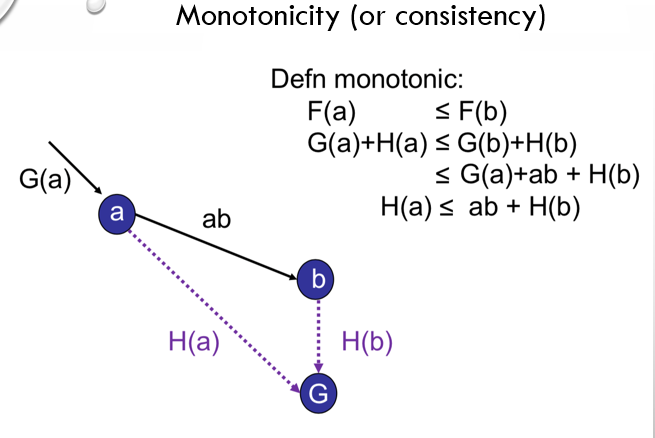
as shown in the slide above if in a given search path we have to travel from state a to a neighboring state b and the difference between H(a) and H(b) is at most the actual distance between the two states then said search path is monotone so instead of defining monotonicity based on F(X) we can define it based on H(X).

now lets test the new deffinition in an example:

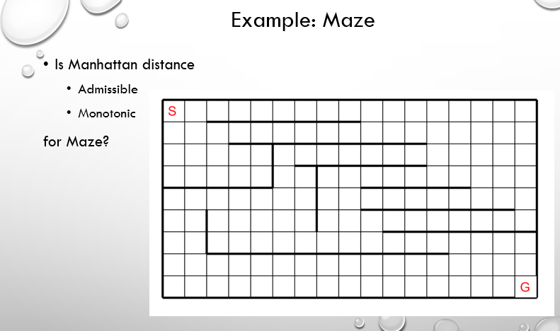
Solution:

now even at first glance we can undrestand that the manhattan distance admissible because we will not be taking the obstacle walls in the middle of the maze into account so the heuristic is always shorter than the actual distance

now regarding the monotonicity of the manhatan distance, imagine two horizontally adjacent states a and b now it's obvious because a and b are adjacent that H(a)-H(b) is either 1 or -1 and the actual distance between a and b is always 1 so H(a)-H(b) is at most the actual distance between a and b hence the manhatan distance heuristic is monotonic.

now lets see another example in the form two heuristics for the 8-puzzle:

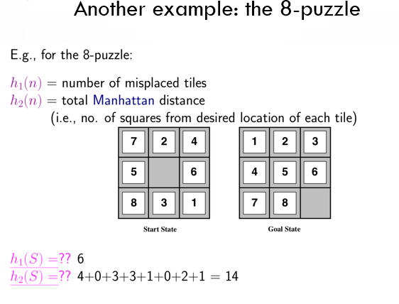
Question: witch of the two demonstrated heuristics is dominant and better to use in the start state?

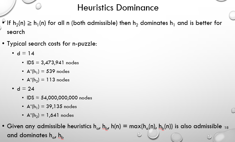
Answer: considering both of the given heuristics are admissible, h1(s) is the dominant heuristic because the ideal heuristic to use in a given state while being admissible has the biggest amount.

note: given a number of admissible heuristics to use in our search the ideal one has the biggest amount

furthermore please look at the figures shown in the slide below:

Relaxed problems: one of the many ways we can aquire heuristic functions is by deriving it from the exact solution cost of a more relaxed version of the problem. keep in mind when we say more relaxed version of the problem what we realy mean is a version of the problem with looser and more relaxed constraints.

Example: previousley the we talked about heuristics h1(n) and h2(n) in the 8-puzzle problem. as is evident we can aquire heuristic h1(n) by relaxing the rules of the 8-puzzle ina way that a tile can move anywhere in the map or similarly we can aquire h2(n) by bending and relaxing the rules of the 8-puzzle so that a tile can move to any adjacent square on the map.

the key point to all this is the optimal solution to a relaxed problem is no greaterthan the optimal solution in the real problem.

another great example of this can be seen in the slide below sorounding the traveling sales person or TSP problem:

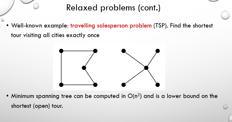
a tour is actually a linear tree with each branch having only one child and starting from a root and eventually reaching a goal now as is shown the np hard TSP problem is initialy an optimization problem in witch the h* is the minimum amount of the sum of the costs of the edges in linear trees we can relax the TSP problem in such a manner that we acquire the minimum sum cost of edges in all trees not just the linear ones and with this act we derive a new heuristic h with ultimately equals the minimum sum of costs of the edges in all trees

Optimality of A(tree search): proving the optimality of A search is fairly easy now considering the subjects covered so far and is handled as such in the slide below:

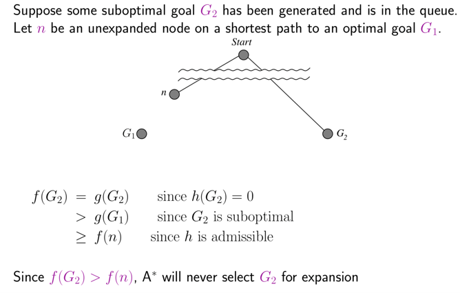
base on the slide above suboptimal goals such as G2 will never be chosen for expantion by the A* in tree search hence rendering A* as a completely optimal algorithem.

now we want to again delve in the subject of monotonicity again and explain why an A* algorithem in a graph search is only optimal if it is in fact monotone. lets explain this with an example in the form ofthe slide below:

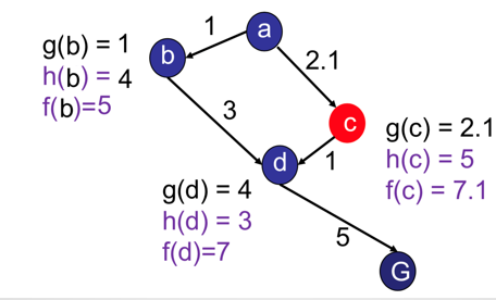
at first glance we can sumize that the optimal path is as follows acdG but if we follow the A* algorithem based on the given f figures we see that the algorithem ultimatley chooses the suboptimal path of abdG this happens becuas node c is never expanded in the algorithem due to f(c) > f(d) and c cannot be expanded untill d is expanded and G is reached in other words f decreases from c to d and is not monotonic hence the suboptimal path is chosen

based on this example we can conclude that in order for the A* to be optimal in a graph search monotonicity is required.

now lets delve in the subject of optimality of A* some more with the demonstrated lemmas in the slide below:

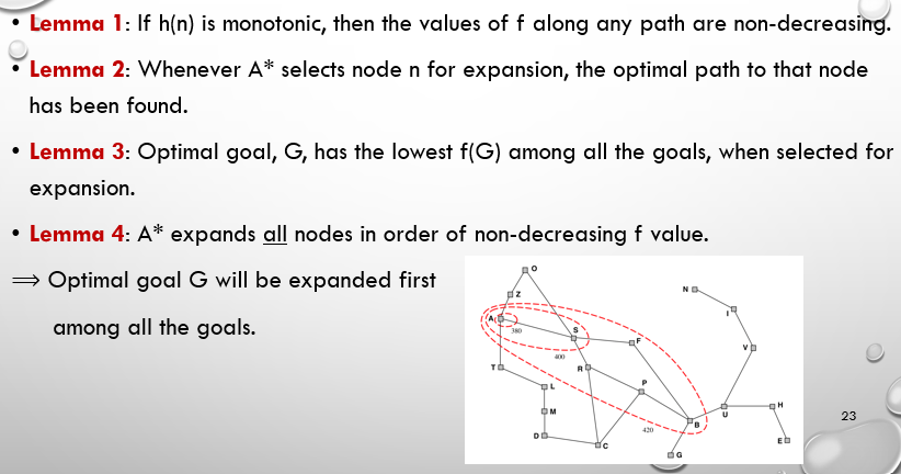
now even at first glance all of the lemmas shown above are quite evident all except for lemma number 2 witch is infact the key lemma for proving the optimality of A* in graph search so lets prove lemma 2:

imagine we started down a start state and find ourselves expanding node n but the path we've chosen turns out to be suboptimal and there is an optimal path for us to choose in order to reach n and the last node stored in the fringe in the optimal path is node m and has not yet been chosen for expantion now because m is in the optimal path from s to n, then g(n) > g(m) + (optimal actual distance from m to n or mn) now lets assume there are k states between m and n considering the heuristic used in this A* is monotonic we can come to the conclusion that: h(m) <= h(m1) + mm1, h(m1) <= h(m2) + mm2, . . . h(mk) <= h(n) + mkn

now we can see that the sum of the above statements is:

h(m) <= h(n) + mn and we previousley mentioned that : g(n) > g(m) + mn using both statements we see that: g(n) + h(n) > g(m) + h(m) witch translates to f(n) > f(m) witch contradicts our initial hypothesis

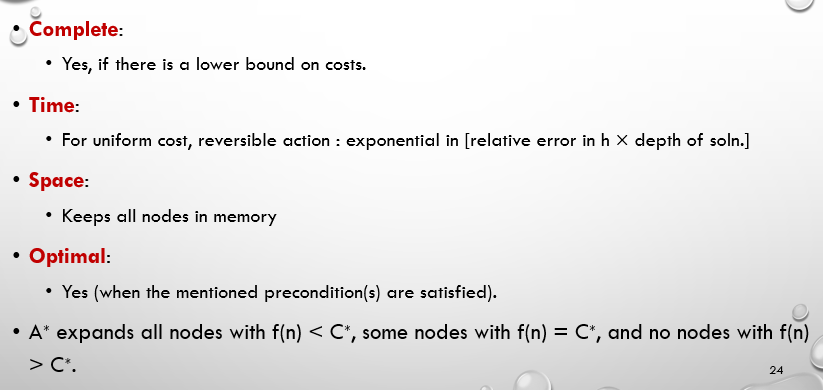
now let us see the properties of A* in the form of the slide below:

A* example:

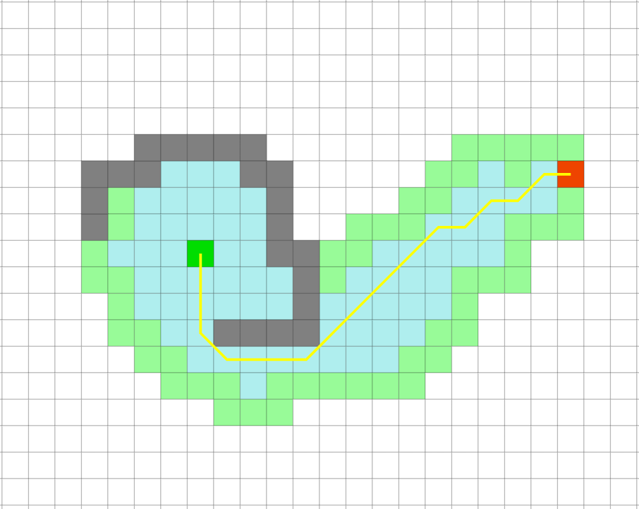
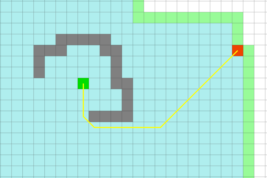
In this example A* algorithm does not work very well until it reaches the wall, and in this special example, it is not very different from the bfs, but when it

crosses the obstacle, it is very fast and clear how clear this algorithm is. In the image below, you can see the A algorithm and BFS algorithm

This example illustrates the importance of accurate heuristic The heuristic is not accurate until it reaches the wall, and it will not be accurate until we cross

the obstacle. The whole advantage is for when we overcome the obstacle So this show us that we need to design good heuristic.

A* summary

Advantages:

It is complete and optimal.

It is the best one from other techniques. It is used to solve very complex problems.

It is optimally efficient, i.e. there is no other optimal algorithm guaranteed to expand fewer nodes than A*.

Disadvantages:

This algorithm is complete if the branching factor is finite and every action has fixed cost.

The speed execution of A* search is highly dependant on the accuracy of the heuristic algorithm that is used to compute h (n).

Exponential growth will occur unless |ℎ(𝑛)−ℎ∗ (𝑛)|≤𝑂(log⁡〖ℎ∗ (𝑛)〗 )

Optimal Efficiency:

Among all optimal algorithms that start from the same start node and use the same heuristic h, A∗ expands the minimal number of paths.

problem: A∗ could be unlucky about how it breaks ties.

So let’s define optimal efficiency as expanding the minimal number of paths p for which f(p) != f∗, where f∗ is the cost of the shortest path.

Lets assume an algorithm B does not expand a node n which is A* expanded by A*. By definition for this path g(n)+h(n) <= f where f is the cost of the shortest

path. Consider a second problem for which all heuristics values are the same as in the original problem. However, there is a new path to a new goal with total

cost smaller f. The assumed algorithm B would expand n hence never reach this new goal. Hence, B wouldn't find this optimal path. Therefore, our original

assumption that B is optimal is violated.

IDA*

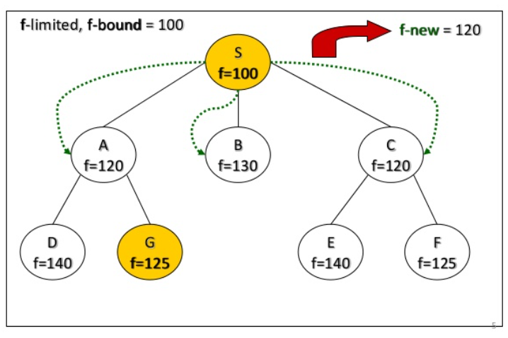
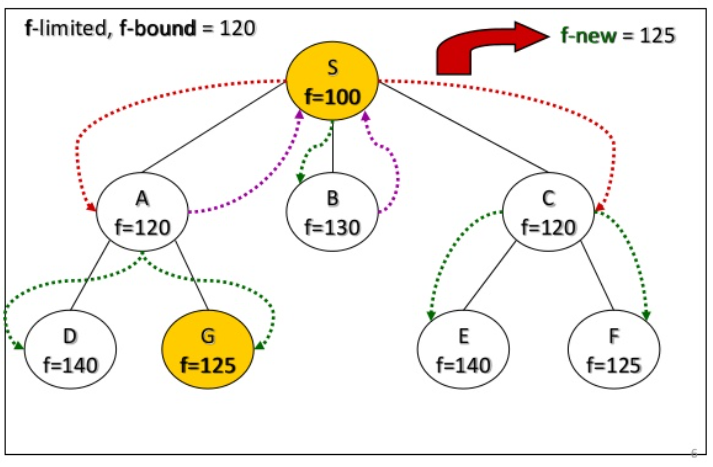
perform deapth-first search limited to some f-bound

if goal found: it's ok

else: increase the f-bound and restart

how to stablish the f-bound?

start with f(start)

Next f-limit = min-cost of any node pruned

IDA* example

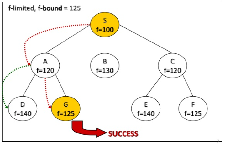
IDA* analyze

IDA* is complete, optimal and optimally efficient

IDA* is complete and optimal space usage is linear in the depth of. each iteration is dfs