Foreword

CNNs are a type of deep learning models are being used a lot in today's world, especially regarding computer vision applications. They can help users in a wide range of possibilities, from recognizing faces and emotions, helping the medical doctors in healthcare settings, aiding students in their education, supporting self-checkout in retail stores, and many more.

Due to their popularity, it seems to be a necessity to learn about how they work and how can we train one using libraries which are now commonplace among researchers and students.

The structure of this notebook is as follows: first, an introduction to CNN is given, then the concept of convolution is described in further details. Afterwards, a CNN model has been trained step-by-step using TensorFlow - a popular framework for ML and vision related activities. Finally, after concluding what we've learned, links are provided for further reading in case you, as a reader, are interested. We assume you know about deep learning and multi-layered ANNs before you start reading this notebook.

So, let's dive in!

Introduction: What is a CNN?

As we know, there are various types of multi-layered artificial neural networks (also called ANNs) available. Specifically, one type of them are called "convolutional neural networks" - or CNNs - which are mostly used in the field of computer vision. They are able to find (or "extract") many features of the images given to them as the training data, and then classify the test dataset by inspecting them for the extracted features.

Numerical representation of an image

It is obvious that computers can't see an "image" as we do; instead, all computer programs work with numbers and digits. As a result, we - as the users of a CNN - should also give it the images we have in a numerical format, or else it won't understand a bit about the image.

Fortunately, we don't need to implement some fancy algorithm to be able to convert an image to a numerical format used by CNNs, because the numbers are already there in format of pixel values. Each pixel is assigned a value in a picture, which are rendered together on a computer screen.

The main problem with this approach is the number of pixels in a picture. An example 128*128 image - which is considered so small in modern measurements - contains 16384 pixels which are usually a lot for a model to find features in. To fix this problem which is common in pre-CNN networks, some new concepts are used in this model.

To continue our discussion onto how the CNNs work, first we should know the concept of convolution. If you know what a convolution is, you may skip the section in which the concept of conclusion and its relation to convolutional neural networks are covered and discussed.

What is a convolution and how do CNNs work?

As we learned till now, we need a way to somehow select the important features in an image while training the model.

You have possibly seen "filters" in the camera app in your smartphone. Many of these filters focus on special parts of your image; as an example, filters such as the "Stage Light" filter in the Camera app in iOS only focuses on your face and blurs the background while taking a pictures. We want to use a similar idea to find features in images here, too.

When talking about CNNs, the filters are usually called "kernels". They are a special kind of matrix (usually 3*3) which is "convoluted" with the matrix of all pixels of the original image. The result of the "convolution" process - which is a mathematical operation - is known as a "feature map" or "activation map".

The details on how the "convolution" is calculated is not necessarily needed in order to understand how to train a CNN using Tensorflow, but an overview is given here.

The convolution operartion works as follows: the kernel will slide over the matrix of the image and an "element-wise" multiplication will happen at every stage. The results of the element-wise multiplication are added together and stored in one pixel of the output matrix.

An example is being presented in the animation below:

Convolution Example

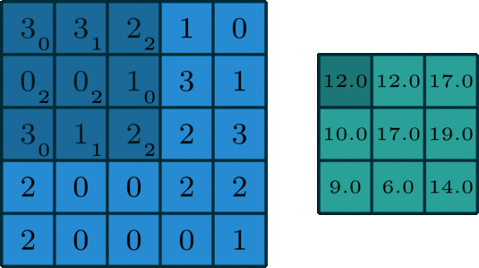
When a convolution is performed, a matrix is transformed into some another matrix. Calculating the weighted some of neighboring cells allows us to only see the input features coming from "about the same" location, instead of exact parameters, which will decrease the number of parameters the model has to train on, to a great extend and as a result, the model can do more iterations or calculations in the same time, possibly leading to a better accuracy on the test data.

Other steps before giving data to the model

Now that we know the basics of convolution, let's discuss a bit more about CNNs in detail.

After the convolution result (feature map) is obtained, we apply a ReLU (Rectified Linear Unit) to make the operation non-linear (as we did in many cases in ANNs). Then, we can use "pooling", another technique in CNNs which ensures the network can find features independent from their location.

A famous type of pooling is called "max pooling" in which the largest value in 2*2 boxes over the picture are selected, as can be inspected in this picture:

Max Pooling Example

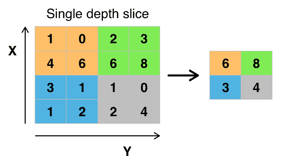
This action will keep the main features while the size of picture is decreased, so possibly there would be less overfitting when the model is being trained.

After pooling is performed on a picture, the matrix is ready to be flattened into a single vector which is able to help the model train.

CNN Architecture

Many architectures regarding CNNs have been previously tried and tested, such as MobileNet, Xception, etc. They have been trained on a dataset of more than a million images, so they include weights in advance which can be used or not (we may use the trained model, or we may only use the architecture and train it again on our own data). Designing a new architecture is also obviously possible.

Train a CNN model using Tensorflow

In this notebook, we want to choose Xception as the architecture to go with. First we start by installing and importing the necessary libraries:

In [7]:

# Import the TensorFlow framework
import tensorflow as tf

We will use Keras to make the model.

If you wonder what Keras is, it is a API for TensorFlow which gives the developers high level access to TensorFlow features and functions. Keras is also included in TensorFlow and will help us build models faster.

In other words, Keras depends on TensorFlow (or some other similar library), but not vice-versa. Keras is an abstraction mostly working on top of TensorFlow. While this makes it easier to accomplish the deep learning tasks, we might lose access to more complex functionalities and utilities.

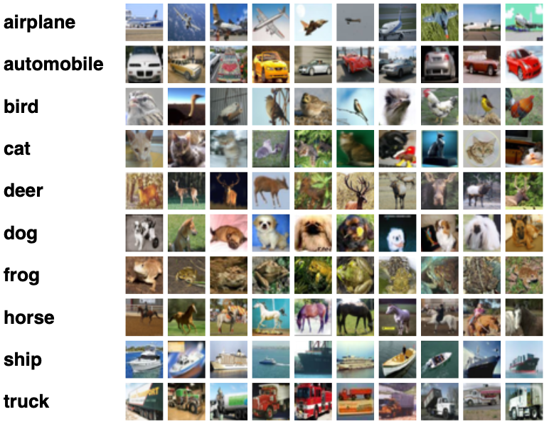
Before going on to make the model, we should import our data. The data is usually collected by a user study and then passed into a model. Here, we use a previously collected dataset called CIFAR10 which is included in Keras itself. This dataset consists of 60000 images of size 32*32, distributed equally in 10 main classes. 10000 of them are test data. Below are some examples of the data in the dataset:

CIFAR10 examples

Now we load the data separately into test and train datasets (X refers to the pictures and Y to the classes). Note that the next line make take a while to execute, depending on the status of your internet connection, because it has to download the dataset from the server the first time you run this line of code.

In [8]:

# Load data from CIFAR10 dataset
# - Xtrain: training pictures
# - Ytrain: training classes
# - Xtest: test pictures
# - Ytest: test classes

(Xtrain, ytrain), (Xtest, ytest) = tf.keras.datasets.cifar10.load_data()

The pixel values are from 0 to 255, so we scale them:

In [9]:

# Scaling the pixel values of the pictures (by a vector element-wise division)
Xtrain = Xtrain / 255
Xtest = Xtest / 255

Now we create a model:

In [10]:

model = tf.keras.Sequential([
    tf.keras.layers.Conv2D(32, (3, 3), activation = "relu", padding= 'same', input_shape = (32, 32, 3)), # Convolution Layer
    tf.keras.layers.MaxPooling2D((2, 2), strides = 2), # Max Pooling Layer
    tf.keras.layers.Conv2D(64, (3, 3), activation = "relu", padding = 'same'), # Convolution Layer
    tf.keras.layers.MaxPooling2D((2, 2), strides = 2), # Max Pooling Layer
    tf.keras.layers.Flatten(), # Flatten Layer
    tf.keras.layers.Dense(200, activation = "relu"), # Dense Layer
    tf.keras.layers.Dense(200, activation = "relu"), # Dense Layer
    tf.keras.layers.Dense(10, activation = "softmax") # Dense Layer
])

model.summary()

Model: "sequential_1"
_________________________________________________________________
 Layer (type)                Output Shape              Param #   
=================================================================
 conv2d_2 (Conv2D)           (None, 32, 32, 32)        896       
                                                                 
 max_pooling2d_2 (MaxPooling  (None, 16, 16, 32)       0         
 2D)                                                             
                                                                 
 conv2d_3 (Conv2D)           (None, 16, 16, 64)        18496     
                                                                 
 max_pooling2d_3 (MaxPooling  (None, 8, 8, 64)         0         
 2D)                                                             
                                                                 
 flatten_1 (Flatten)         (None, 4096)              0         
                                                                 
 dense_3 (Dense)             (None, 200)               819400    
                                                                 
 dense_4 (Dense)             (None, 200)               40200     
                                                                 
 dense_5 (Dense)             (None, 10)                2010      
                                                                 
=================================================================
Total params: 881,002
Trainable params: 881,002
Non-trainable params: 0
_________________________________________________________________

Here are what the layers mean (activation is ReLU in all cases except the last which we want a discrete, multi-class output from and Softmax is used instead):

Conv2D is the layer related to the convolution operation.
- The kernel is assumed to be 3*3.
- Number 32 in the parameters came from the size of the input pictures, which were 32 by 32.
- The value "same" for padding will result in a photo of a same size while doing the convolution by adjusting the padding. You can learn more about the padding here if you wish.
MaxPooling2D is the layer related to the max pooling operation. The size of the pooling window ((2, 2)) and the stride (number of steps) define the size for the next layer to be 64.
There is another pair of the aforementioned layers used (no limit in usage, but usage of more layers will take the model longer to learn).
To be able to feed the data into dense layers, we should first flatten the data using Flatten.
Three dense layers are used. The most important thing to note of them is the first parameter of the last layer should obviously be equal to the number of prediction classes, which is 10 in case of CIFAR10.

Now we train the model. The process is similar to what we have in ANNs in TensorFlow.

In [11]:

# Compile the model prior to fitting it on the training data and testing it on the validation data
model.compile(optimizer = 'adam',
              loss = tf.keras.losses.SparseCategoricalCrossentropy(from_logits = True),
              metrics = ['accuracy'])

In [ ]:

# Fit the model to the training data
# - 500 epochs (iterations)
# - also validate the model on the test data
history = model.fit(Xtrain, ytrain, epochs=500, validation_data = (Xtest, ytest))

And we can easily plot the loss and accuracy:

In [ ]:

# Import Pandas library which helps us in the rest of the code of this blokc
import pandas as pd
# convert the history object from the result of the fit function into a Pandas dataframe
history_items = pd.DataFrame(history.history)

# Plot the loss and the accuracy of the model (both the training and the validation loss and accuracy)
history_items[["loss","val_loss"]].plot()
history_items[["accuracy","val_accuracy"]].plot()

How to improve the model

Although the model works in this state, there are various actions one might perform in order to make it better in real-world problems and tests. In this section, we are discussing various attempts at making the model perform better and with more correct predictions.

Dropout regularization

Model architects sometimes add the functionality to drop some of the connections of the model in the training, because this will lead the model to avoid memorizing input data. By removing some connections, a model that has memorized inputs will produce a noticable amount of wrong results, but a model that has really "learned" the data performs well. We can easily add a dropout layer with a certain rate, like the following: (the layer just before the last is the dropout layer)

In [ ]:

# Example to demonstrate how can we add dropout regularization to the model
# The model is the same as the first model in this notebook, except for the dropout layer being added

model = tf.keras.Sequential([
    tf.keras.layers.Conv2D(32, (3, 3), activation = "relu", padding= 'same', input_shape = (32, 32, 3)),
    tf.keras.layers.MaxPooling2D((2, 2), strides = 2),
    tf.keras.layers.Conv2D(64, (3, 3), activation = "relu", padding = 'same'),
    tf.keras.layers.MaxPooling2D((2, 2), strides = 2),
    tf.keras.layers.Flatten(),
    tf.keras.layers.Dense(200, activation = "relu"),
    tf.keras.layers.Dense(200, activation = "relu"),
    tf.keras.layers.Dropout(0.25), # Dropout layer
    tf.keras.layers.Dense(10, activation = "softmax")
])

model.summary()

Batch Normalization

Normalization, in general, means to transform the data (the numbers) to a pre-set, common scale, while the general shape of the distribution remains the same. The main goal of normalization is to make model able to generalize, or faster. It has been seen that by normalizing the data to have a mean of zero and a standard deviation of one, the model would run faster. This process is called "batch normalization" and will make the model train faster.

The part "batch" in the name refers to the sets of data on which the model is trained. So, the normalization happens on batches and not on single points of input data.

Batch normalization also offers regularization, so it is advised that we use either batch normalization or dropout regularization and not both simultaneously.

Adding batch normalization as a layer is so simple. The following example shows how can we do this. (The layer just before the last is the batch normalization layer)

In [ ]:

# Example to demonstrate how can we add batch normalization to the model
# The model is the same as the first model in this notebook, except for the batch normalization layer being added

model = tf.keras.Sequential([
    tf.keras.layers.Conv2D(32, (3, 3), activation = "relu", padding= 'same', input_shape = (32, 32, 3)),
    tf.keras.layers.MaxPooling2D((2, 2), strides = 2),
    tf.keras.layers.Conv2D(64, (3, 3), activation = "relu", padding = 'same'),
    tf.keras.layers.MaxPooling2D((2, 2), strides = 2),
    tf.keras.layers.Flatten(),
    tf.keras.layers.Dense(200, activation = "relu"),
    tf.keras.layers.Dense(200, activation = "relu"),
    tf.keras.layers.BatchNormalization(), # Batch normalization layer
    tf.keras.layers.Dense(10, activation = "softmax")
])

model.summary()

There is an important note which is nice to know when you are using batch normalization. While we are in the "training" phase, the mean and SD of the current data is used, but when we are in the "predicting" phase, the data obtained from training is used, because those weights are what has made the model and bu changing the weights of this layer on a pre-trained model, the learned data would be lost or damaged.

Conclusion

In this notebook, we learned what a CNN is and why do we need one. In addition, the main concept behind CNNs, which is the convolution, was described. The concept of kernel was also defined, and how can we treat a picture numerically was described in details.

Then, we practiced different steps needed in order to train a CNN model, especially using ReLU and also pooling. A dataset called CIFAR10 was introduced, which is a good starting point for who wants to get their hands dirty with CNNs.

After that, the steps to train a CNN using TensorFlow was mentioned one after another, and finally, some suggestions to improve the results of the prediction (dropout regularization and batch normalization) were defined, described and used in code examples.

Extra suggestion: Save the model

Because training CNNs takes a lot of time, when experimenting with the results of the model, it's usually better to save the model for further usage.

In [ ]:

path = "....." # fill this with your own path
model.save(path) # save the model

Convolutional Neural Networks

Foreword

Introduction: What is a CNN?

Numerical representation of an image

What is a convolution and how do CNNs work?

Other steps before giving data to the model

CNN Architecture

Train a CNN model using Tensorflow

How to improve the model

Dropout regularization

Batch Normalization

Conclusion

Extra suggestion: Save the model

Further reading and references

Seyed Parsa Neshaei