Decision Tree Learning

What Is a Decision Tree?

Decision tree learning is a method commonly used in data mining. The goal is to create a model that predicts the value of a target variable based on several input variables.

A decision tree is a simple representation for classifying examples. For this section, assume that all input features have finite discrete domains, and there is a single target feature called the classification. Each element of the classification domain is called a class.

A decision tree, or classification tree, is a tree in which each internal node is labeled with an input feature. The arcs leaving that node are labeled with possible values of that feature, or they lead to another decision node. Each leaf is labeled with a class or a probability distribution over classes, meaning the dataset has been classified into either a specific class or a class distribution.

Overview

Decision Tree Examples

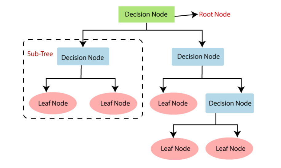
Decision trees can describe simple, explainable classification rules.

Accepting a New Job Offer

Predicting Fuel Efficiency

Building a Decision Tree

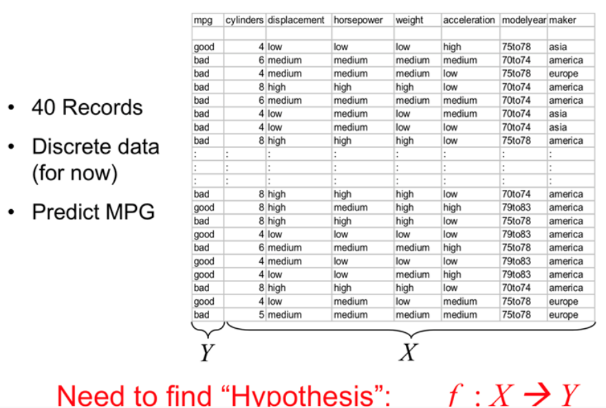
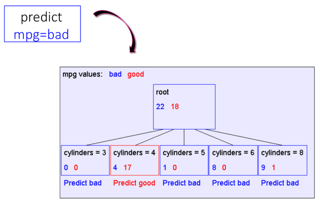
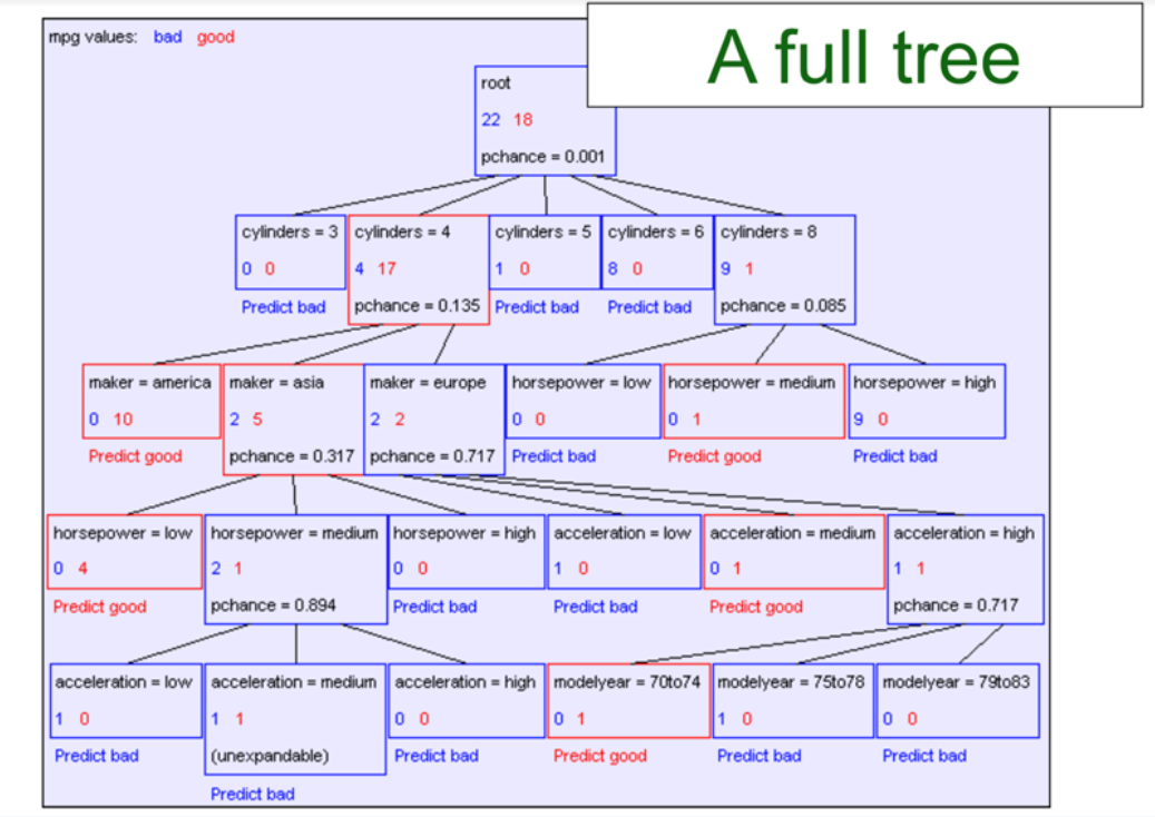
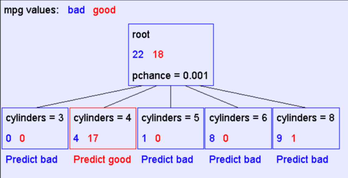
Now we build a decision tree for the fuel-efficiency example.

Starting Node

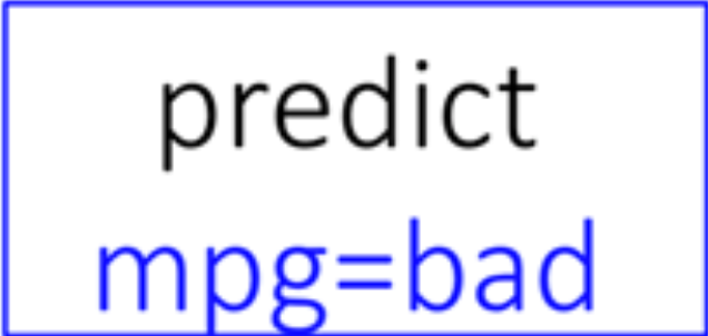
We can start with an empty tree and improve it at each level. For the fuel-efficiency example, suppose the initial tree returns mpg = bad for all data points. On this dataset, that tree gives 22 correct answers and 18 wrong answers, so there is room to improve it.

Operators

There are several operators for building a decision tree.

Improving the Tree

To improve the tree, we can add more nodes, or features, to make better predictions.

Recursive Step

We can consider each leaf as a root and repeat the same splitting process. Sometimes we reach a node that does not have any data. In that case, we should stop and predict randomly or fall back to a default rule.

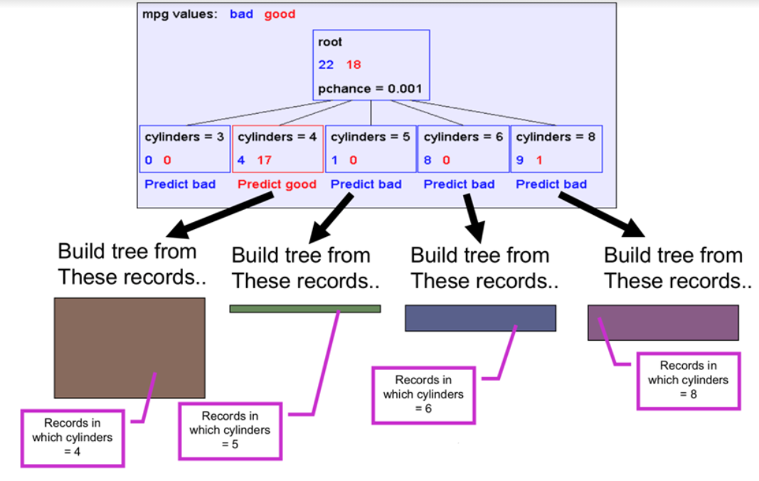
After one level, we get this tree:

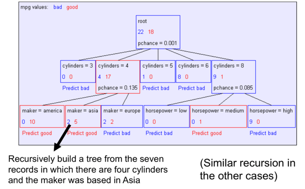
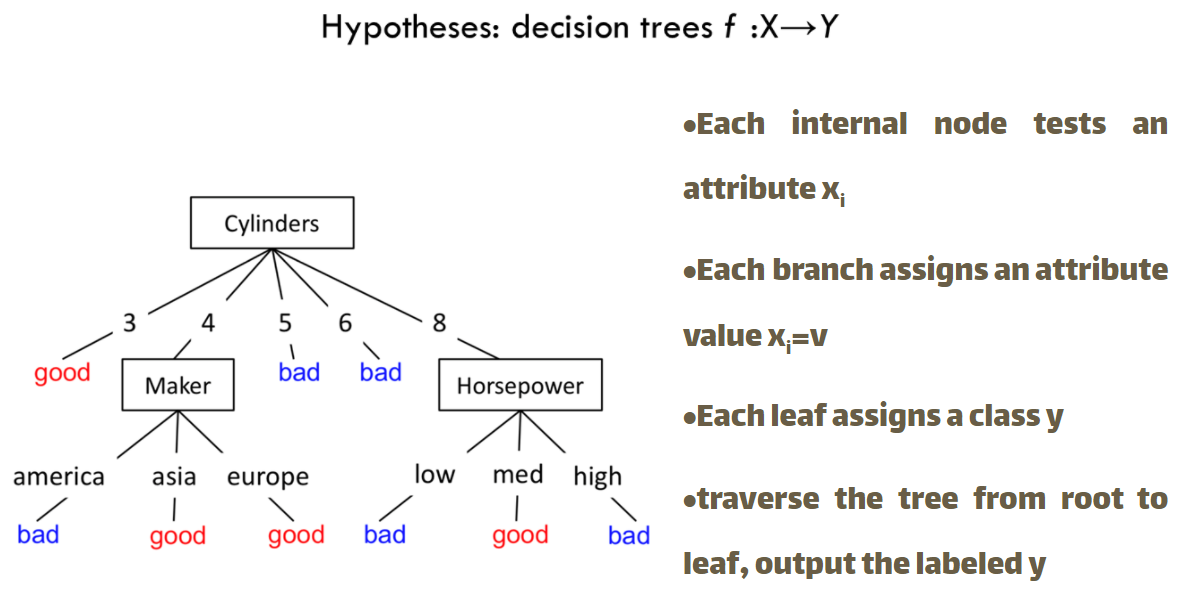
After adding all nodes and features, we get a full tree:

Two Questions for More Efficiency

A basic hill-climbing strategy for decision trees is:

• Start from an empty decision tree.
• Split on the best attribute or feature.
• Recurse on the resulting subsets.

The important questions are:

• Which attribute gives the best split?
• When should recursion stop?

Splitting: Choosing a Good Attribute

Look at the example below to see the main idea behind splitting.

Measuring Uncertainty

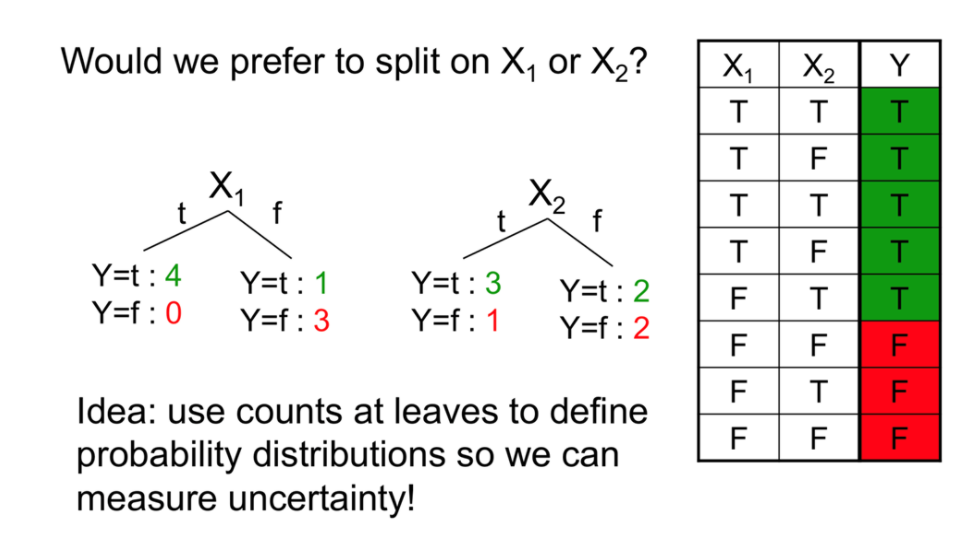
A split is useful when we become more certain about the classification after the split.

• Deterministic splits are good: all true or all false.
• Uniform distributions are bad: the split did not make the outcome clearer.

Which Attribute Gives the Best Split?

Two common answers are:

• Use the attribute with the highest information gain, defined in terms of entropy.
• Use another objective, such as accuracy, to reduce the misclassification rate.

Entropy and Information Gain

Entropy

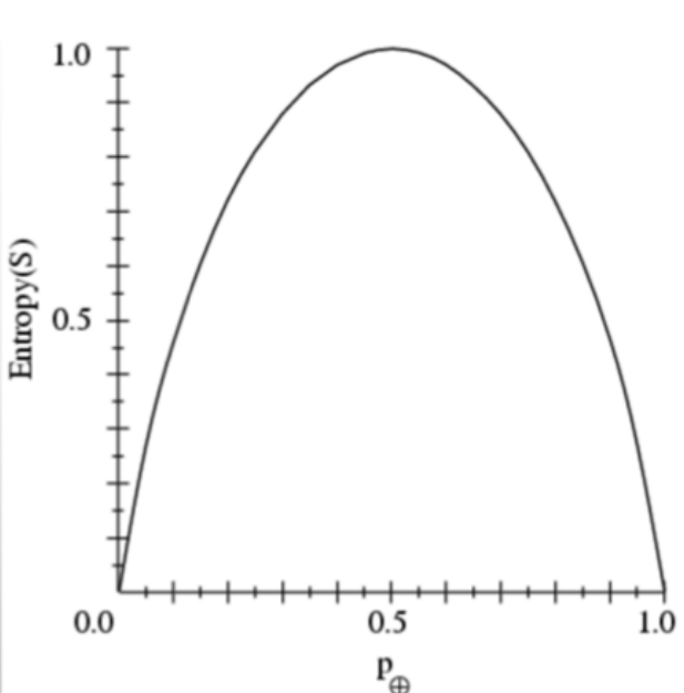
Entropy measures uncertainty in a random variable. More uncertainty means more entropy.

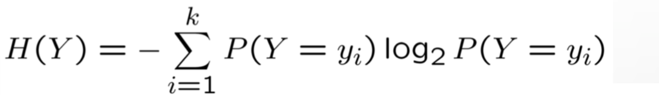
In information theory, entropy is the expected number of bits needed to encode a randomly drawn value of a variable under the most efficient code. Diagrammatically, entropy peaks in the middle and falls near deterministic outcomes.

Example of Entropy

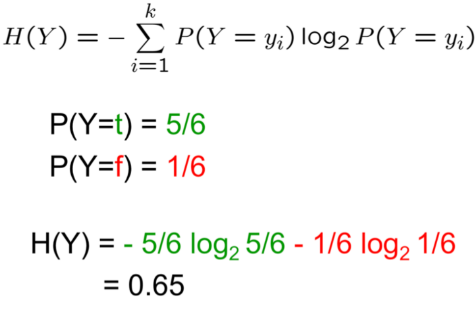
If P(Y = t) = 5/6 and P(Y = f) = 1/6, the value of H(Y) is:

Conditional Entropy

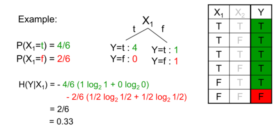
Conditional entropy H(Y | X) measures the uncertainty of a random variable Y after observing another random variable X.

Here is an example of conditional entropy:

Information Gain

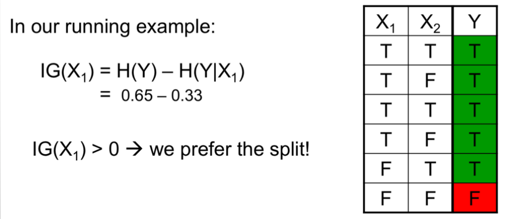
Information gain is the amount of information gained about one random variable or signal from observing another random variable.

For the previous example, the information gain is:

Learning a Decision Tree

When learning a decision tree, we need to decide:

• Which node to split.
• How to update the tree after each iteration.
• Which termination condition to use.

A common learning procedure is:

• Start from an empty decision tree.
• Split on the next best attribute or feature.
• Use information gain, or a related score, to select the attribute.
• Recurse.

Example

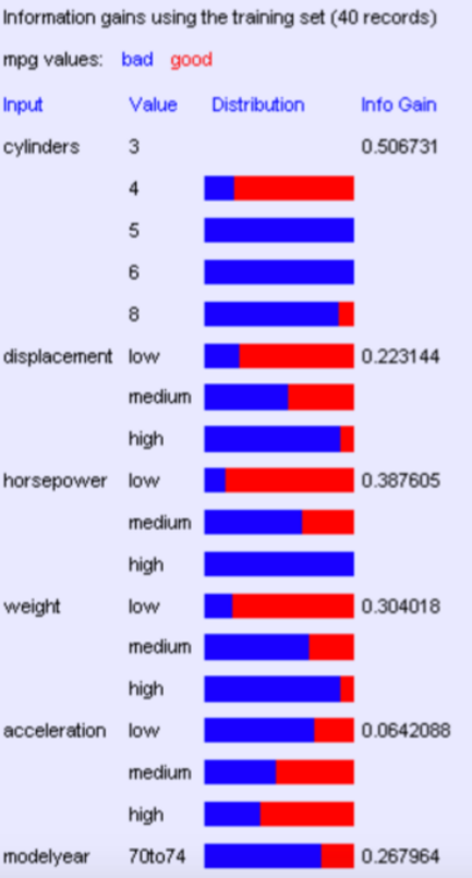
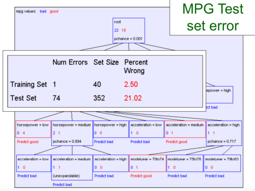
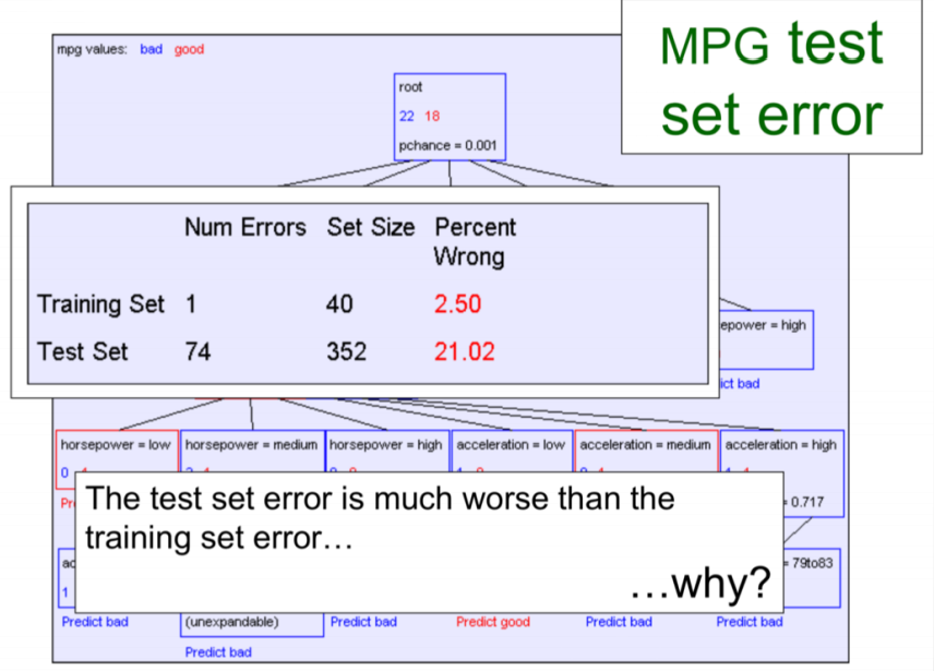
Suppose we want to predict MPG. First, we inspect the information gains for possible splits:

Then we start iterating. For the first iteration we have:

Continuing the process gives:

Termination Conditions

Termination conditions tell us when to stop growing the tree.

Two basic termination rules are:

• Base case one: If all records in the current data subset have the same output, do not recurse.
• Base case two: If all records have exactly the same input attributes, do not recurse.

Base Case One

Base Case Two

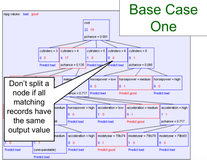
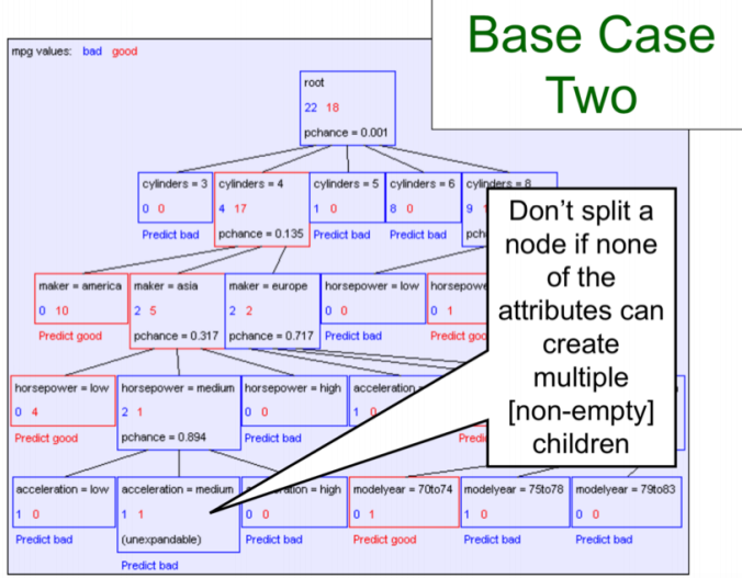
A third tempting rule is:

• Base case three: If all attributes have zero information gain, do not recurse.

Is that a good idea? Not necessarily. It is greedy: it checks variables alone, but a combination of variables may still contain useful information.

For Y = a xor b, this rule gives:

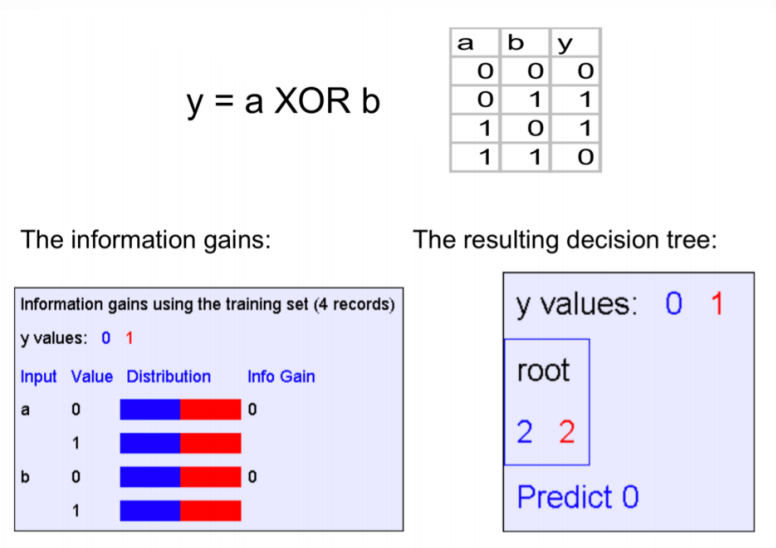
Without that rule, we can still find the useful structure:

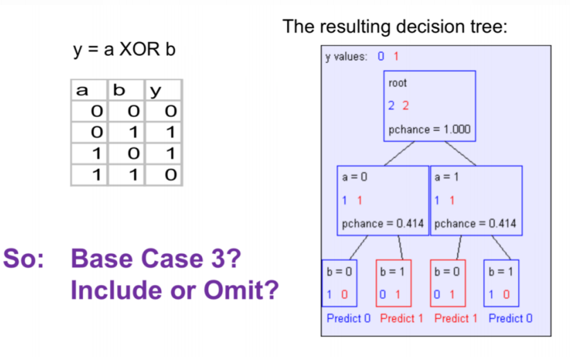
So this stopping rule may produce a poor result:

Overfitting in Decision Trees

Decision trees have little learning bias, which can make their variance over the training set significantly high. How can we introduce useful bias to reduce overfitting?

No Free Lunch Theorem

Consider the graph below. Suppose we are given a dataset of (x, y) points and want to estimate the function that generated them.

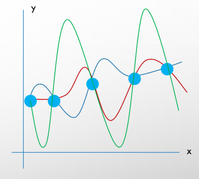
All three functions, red, green, and blue, fit the data. Without prior knowledge, all three have the same probability of being the suggested function.

The No Free Lunch theorem says that without any sense of which functions are more likely, learning is impossible. For example, if we already knew that a very smooth function generated these points, we would prefer the blue function over the others.

Occam's Razor

Occam's Razor says that among all possible hypotheses for a dataset, we should prefer the shortest or least complex one, because a shorter hypothesis is less likely to overfit.

Variance of a Model

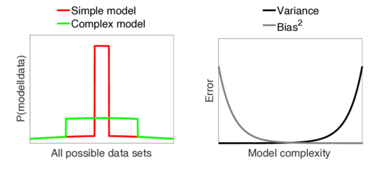
Variance measures how much the result on a validation set changes if we change the training data.

Bias of a Model

Bias measures the deviation introduced from the original training data while training.

According to Occam's Razor, we would rather build smaller trees with less depth.

How to Build Small Trees

There are two common approaches.

Stop Growing Before Overfitting

• Bound the depth or number of leaves.
• Stop growing if the information gain of all remaining features is zero at a depth.

Grow the Full Tree, Then Prune

• Optimize on a held-out validation set.
• After training, prune any branches that do not reduce validation accuracy below a threshold.
• This usually requires a larger amount of data.
• Statistical significance testing can also help decide what to prune.

Statistical Significance Testing

Chi-Square Test Reminder

Suppose we have two features: the first has k classes and the second has n classes. Given people whose classes are known for both features, the null hypothesis states that in a table with k rows and n columns, rows are independent from columns, and vice versa.

Using Chi-Square While Growing a Tree

For choosing which feature to use at each depth, we used information gain. After the tree is grown, either fully or with a limit on depth and leaves, we can test each feature at each depth and calculate a p-value.

After setting a threshold called MaxPchance, if the calculated p-value for any feature is greater than MaxPchance, we prune that feature and make the decision based on the previous feature, or parent node.

How to Find a Good MaxPchance

We can use local or greedy search on the validation set. Once we reach good validation accuracy, we stop and set that value as MaxPchance.

Additional Content: Random Forests

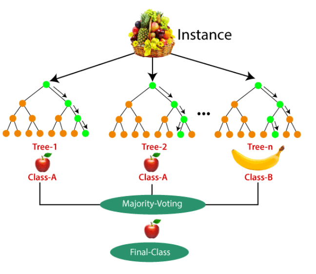
Decision trees overfit easily, and it is hard to grow them on a large number of features. Random forests address this by using multiple decision trees instead of only one.

Training Set

Assume T is the original training set. It is not usual to divide it into N disjoint subsets, where N is the number of decision trees in the forest. To reduce overfitting, we choose a subset size of phi_1 |T|, then bootstrap, or bag, T into N subsets of size phi_1 |T|, where 0 < phi_1 <= 1.

Features

One problem with a single decision tree is that it is hard to grow on many features. In a random forest, we randomly choose a subset of features with size phi_2 |F| and assign it to each tree, where 0 < phi_2 <= 1.

Prediction

There are two common ways to report the final prediction for each test sample.

Max Method

Report the class predicted most often. For example, if 3 out of 5 trees predict Y = 1, report Y = 1.

Properties:

• Lower F1 score.
• Higher recall.
• Lower precision.
• Needs a random tie-break when the number of trees is even.

Average Method

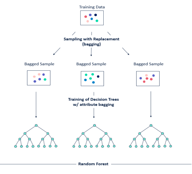
Each tree reports a prediction and a confidence probability. We calculate a weighted average of each tree's prediction, using the reported probabilities as weights.

Properties:

• Higher F1 score.
• Lower recall.
• Higher precision.
• More reasonable behavior when the number of trees is even.