Mehrshad Mirmohammadi
Author
In regression, we have some data points and a number or a label is assigned to each data point. Our goal is to predict the number or label of an unseen data point after learning from the data we already have. We assume each data point is a vector $x$ and we want to predict $f(x)$. The first idea is to use interpolation. By using interpolation, we will have a high degree polynomial that fits our training data perfectly. But the problem is that interpolation leads to overfitting. So the error for unseen data will be too large. In regression, we aim to find the best curve with a lower degree. Although there will be some training error here, our test error will decrease since we are avoiding overfitting.
Here, we want to assign $f(x)$ to each data point $x$. In linear regression, we assume $f$ is a linear function. We can define $f$ as
$$ f_w(x) = w^T x = \begin{bmatrix} w_0 & w_1 & \cdots & w_n \end{bmatrix} . \begin{bmatrix} 1 \\ x_1 \\ \vdots \\ x_n \end{bmatrix}. $$ We assumed $x_0 = 1$ in $x$ to have bias in our function. So the data points are in an n-dimensional space.
We also define $y$ as
$$ y_w = \begin{bmatrix} f_w(x^{(1)}) \\ f_w(x^{(2)}) \\ \vdots \\ f_w(x^{(m)}) \end{bmatrix} $$ where $x^{(i)}$ is the i'th data point.
After defining $f$, we need to find the best function. By defining a loss function, we can try to minimize loss by changing $w$ in the main function. Assuming $L$ as our loss function, best $f$ will be
$$ \hat{w} = argmin_w L(y_w, \hat{y}) \rightarrow f_{best}(x) = f_{\hat{w}}(x) $$where $\hat{y}$ is the given number for each data point.
The main loss function we use is mean squared error. It's defined as
$$ MSE(y_w, \hat{y}) = \frac{1}{2} \Sigma_{i=1}^m \left[ y_w^{(i)} - \hat{y}^{(i)} \right]^2 . $$ The main reason for using this function is that we can calculate gradients easily. So we can use gradient descent to find $\hat{w}$.
We want to use gradient descent to find $\hat{w}$. First, we need to calculate $\nabla_w L(y_w, \hat{y})$ because it's used in the gradient descent method. The partial derivatives for MSE are:
$$ \frac{\partial MSE}{\partial w_j} = - \Sigma_{i = 1}^m x_j^{(i)} \left[ y_w^{(i)} - \hat{y}^{(i)} \right] $$So for gradinet, we have:
$$ \nabla_w MSE = \begin{bmatrix} \frac{\partial MSE}{\partial w_0} \\ \vdots \\ \frac{\partial MSE}{\partial w_n} \end{bmatrix} $$Now, we can find $\hat{w}$ by the gradient descent algorithm as
$$ w^{(i+1)} = w^{(i)} - \eta \nabla_{w^{(i)}} L $$where $\eta$ is the learning rate.
If we define
$$ X = \begin{bmatrix} x^{(1)} \\ \vdots \\ x^{(m)} \end{bmatrix} $$and solve the equation $\nabla_w MSE = 0$, we get the normal equation. It's defined as $$ \hat{w} = (X^TX)^{-1} X^T \hat{y}. $$ However, for using this equation, our features must be linearly independent. Otherwise, $(X^TX)^{-1}$ is not defined. In that case, we can use the pseudo inverse of $X^TX$ instead of the $(X^TX)^{-1}$. Since the calculation of inverse is computationally inefficient, we usually prefer using gradient descent.
In this section, we want to find the best $P(x)$ where x is a real number and $P$ is an n'th degree polynomial.
We can define $$ z = \begin{bmatrix} x^0 \\ x^1 \\ \vdots \\ x^n \end{bmatrix}, $$ then use linear regression to find $f_w(z) = w^T z$. From definition, we know that $P(x) = f_w(z)$. However, if $n$ is too large, overfitting might happen since we are getting closer and closer to interpolation.
To prevent overfitting, we must try to define $n$ optimally. Since $n$ is a hyperparameter here, we can use validation set.
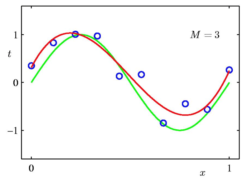
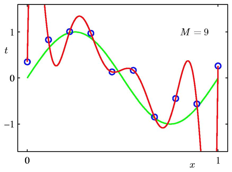
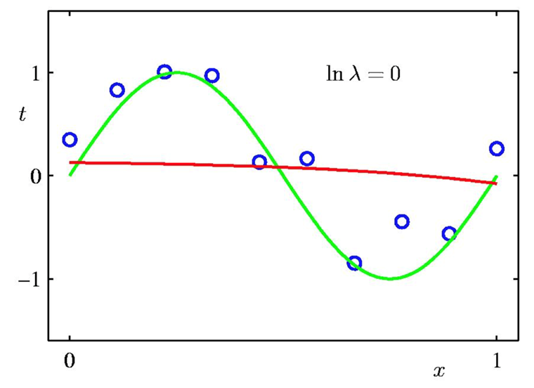
The example below demonstrates how $n$ can change the curve we find and when overfitting happens. The green curve is our goal. The red curve is the M'th degree polynomial using this method.
We split a part of the training data, and don't use it for training. Then, by calculating the loss function over this data, we can optimize $n$. Since the model hasn't seen these data points, we can be sure that overfitting will decrease.
We can see in the above examples that $M = 3$ gives us the best curve. If we compare the validation loss for $M=3$ and $M=9$, the loss will be less for $M=3$ since it's closer to the green curve.
Although using a validation set is a good way to prevent overfitting, We still might try to find the curve which best fits the data, not the curve which best matches it. Regularization tries to make $w$ smaller. The intuition is that large coefficients in $w$ happen because it tries to fit the points. It means that the curve will only get closer to each point. However, decreasing coefficients will make a better curve which might be further from each point, but does a better job at predicting the unseen data.
We only define $l_2-\text{regularization}$ since it's easier to derive and understand. The loss function is
$$ \tilde{E}(y_w, \hat{y}) = \frac{1}{2} \Sigma_{i=1}^m \left[ y_w^{(i)} - \hat{y}^{(i)} \right]^2 + \frac{\lambda}{2}||w||^2 $$ where $\lambda$ is a hyperparameter that controls how small the $w$ should be.
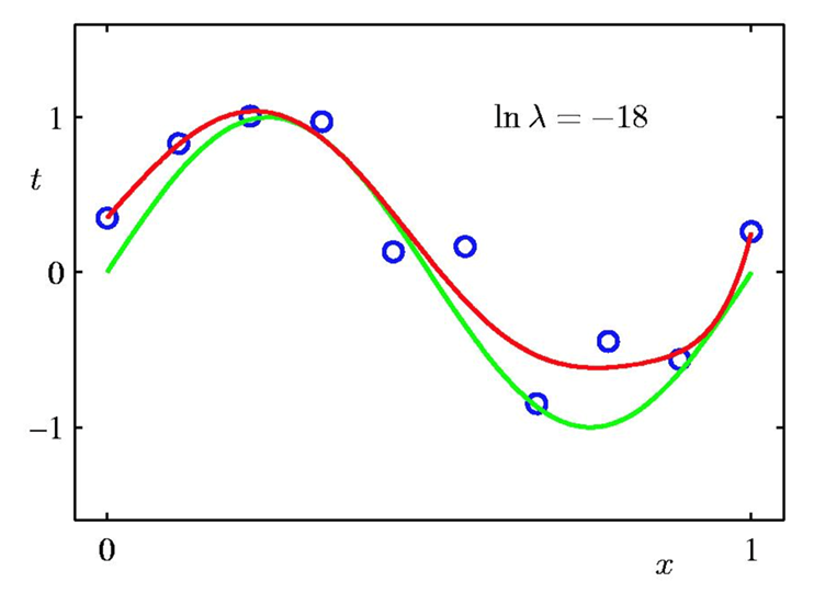
In the following examples, we use regularization with 9'th degree polynomials. We can compare these with the overfitted example above. Also, we can see how important the choice of $\lambda$ is. So, using the validation set might be still useful to optimize $\lambda$.
There are some regression algorithms that can be used for classification (And vise versa). Logistic Regression is one of these algorithms. It can calculate the probability that an instance belongs to a particular class. We can use this probability for classification: if the probability is higher than 0.5 then that instance belongs to the particular class.
Let's start with a simple example. We want to classify flowers that are Iris Virginica from those that are not Iris Virginica. This classification is based on Petal Width and Petal Height. Also, consider that there is some line l (black line in the image below) that separates these 2 types of flowers.
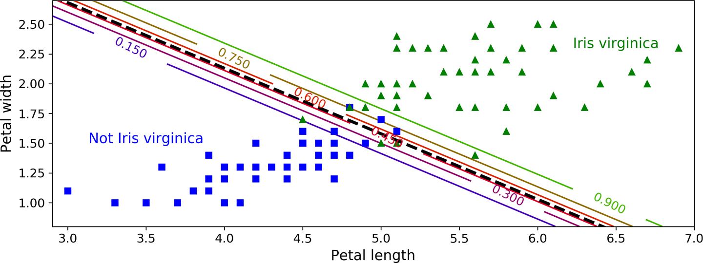
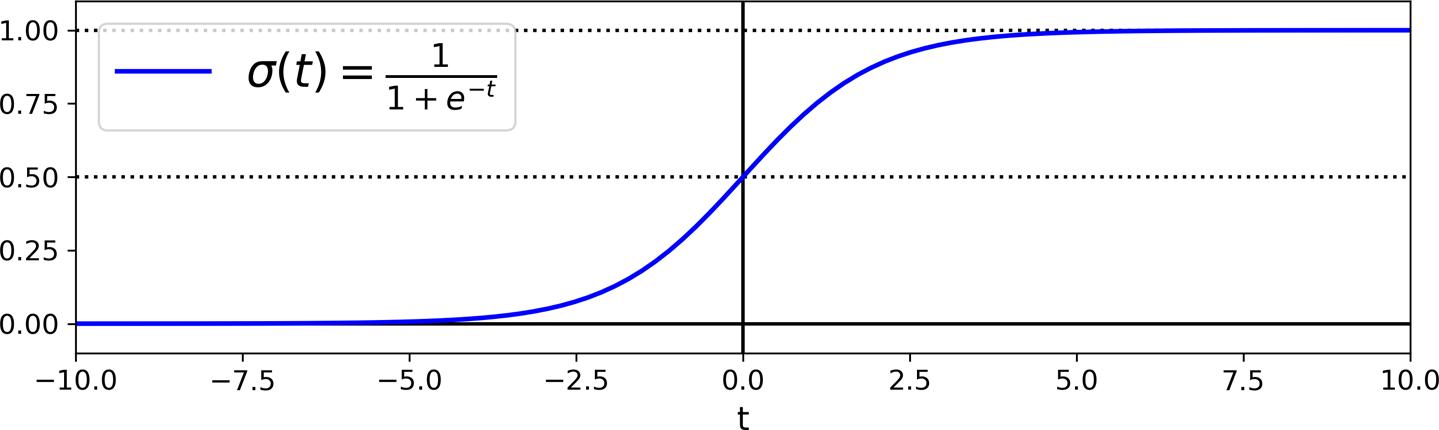
Now, to calculate the probabilities, we use the intuition that, the further we are from l, the higher is the probability of belonging to that particular class. To be more exact, consider we want to find the probability of a given flower being Iris Virginica. Let's call the signed distance between the flower and the line, t. Signed-distance means if we are in the Iris Virginica region, the distance is positive, otherwise, if we are in the not Iris Virginica region, the distance is negative. The probability of this flower being Iris Virginica is related to the value of t, the higher the value of t, the higher the probability. So we need a function $\sigma(.)$ that when given the singed distance t, returns the probability p. The logistic function is a common choice for this purpose. It is a sigmoid function (i.e., S-shaped) that outputs a number between 0 and 1.
Logistic function: $$ \sigma(t) = \frac{1}{1 + \exp(-t)} $$
In the image above, you can see the probability of colored lines. For example, all the points on the green line have a probability of 0.9. These probabilities are calculated using the Logistic function. Also in the image below, you can see the value of the Logistic function for different inputs:
Now that we know how to calculate the probabilities, the problem is reduced to finding the best line l that separates 2 classes. For this, first, we need to define the line and second, we need to define a cost function $J(\theta)$ and then we should find the line l such that it minimizes $J(\theta)$.
We define line l with parameters $\theta$ like before. With this definition, the signed distance between x and the l can be calculated as follows: $$ t_{\theta}(x) = x^{T}\theta $$ Now we can define the probability of a given x with respect to line l with parameters $\theta$:
$$ \hat{P} = \sigma(t_{\theta}(x)) = \sigma(x^{T}\theta) $$We consider that our dataset has N data points $X_i$ with the label $y_i \in \{0 , 1\}$. The cost function for just a single data point can be defined as:
$$ J(\theta) = -log(\hat{P})y -log(1 - \hat{P})(1 - y) $$ where $\hat{P}$ is the probability predicted for this data point given the line l with parameters $\theta$.
And for N data points, we can define cost function as:
$$ J(\theta) = -\frac{1}{N}\sum_{i = 1}^{N}log(\hat{P}^{i})y^{i} -log(1 - \hat{P}^{i})(1 - y^{i}) $$ where $\hat{P}^{i}$ is the probability predicted and $y^{i}$ is the label for the $i^{th}$ data point given the line l with parameters $\theta$.
Unfortunately, there is no known closed-form equation to compute the value of $\theta$ that minimizes this cost function. But the good news is that this cost function is convex! So we can use gradient descent to find the minimum. Because of convexity, Gradient Descent is guaranteed to find the global minimum (with the right learning rate). We can compute the partial derivatives for the $j^{th}$ parameter of $\theta$ as follows:
$$ \displaystyle \frac{\partial}{\partial\theta_{j}}J(\theta) = -\frac{1}{N}\sum_{i = 1}^{N}(\sigma(\theta^{T}x^{i}) - y^{i})x^{i}_{j} $$Regression is used in a variety of AI problems. We can use it to find the best line or curve to predict a function, or to find the best hyperplane dividing 2 classes in a classification problem. In this lecture note, we discussed how to solve these problems and how to prevent overfitting. However, for more complex functions or more classes, you might want to take a look at neural networks.