Markov Decision Processes

Overview

MDP is a model for describing the environments in which an agent is working and trying to achieve a goal, and a series of actions are done to achieve the goal. Markov's presence indicates it is defined on probabilistic space, and the goal is to find an optimal policy that gives the best action in each state to maximize the total amount of rewards.

Grid World Example

Example

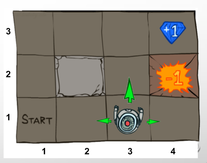
There is a factor in a maze that intends to maximize the sum of its rewards. Every move it makes has a small move cost. In some states, there are rewards and in some states there are fines.

Difference from ordinary search problems

maze environmental uncertainty and The importance of intermediate steps in MDP

Each move selected has a probability of 80% moving in the specified direction and with 10% to the right and with a 10% probability to the left of the specified direction.

Deterministic and Stochastic Transitions

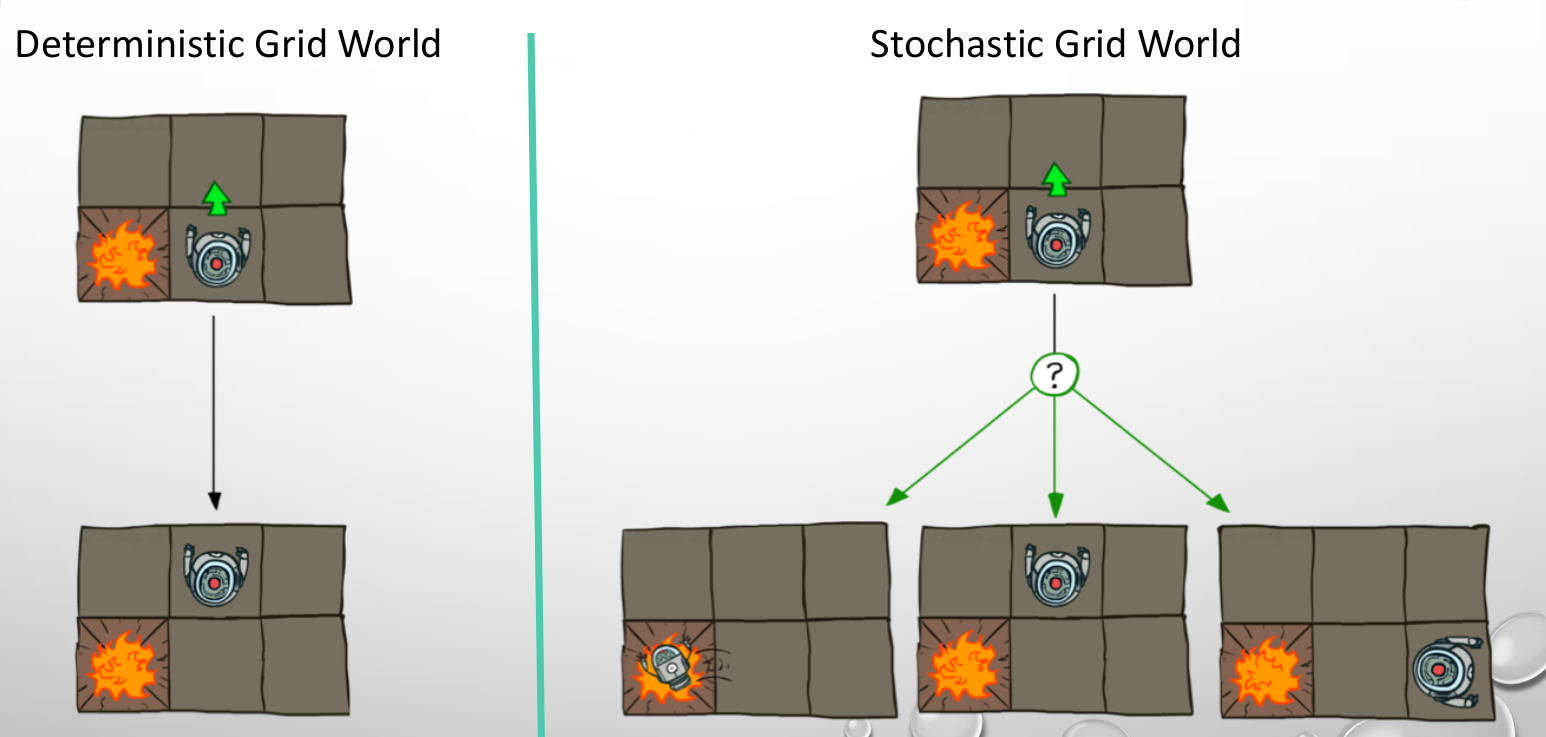
In the deterministic model, every decided move is executed correctly, but in the stochastic, several moves with different probabilities may be executed.

Stochastic example

Actuator error

In a robot system, when a command is given to perform an action and environmental factors can prevent it from moving, it will be like Stochastic, and for example, if the robot wants to move its moving arm but the ground is not flat, the arm might be placed elsewhere. .

For example, if you want to buy stock in the stock market or do not buy at all, there are factors in this market and some of them are visible and some of them are not visible like how macroeconomic policy decisions are made, and if you buy, Because this uncertainty exists, it may result in different behaviors.

MDP Definition

Entities

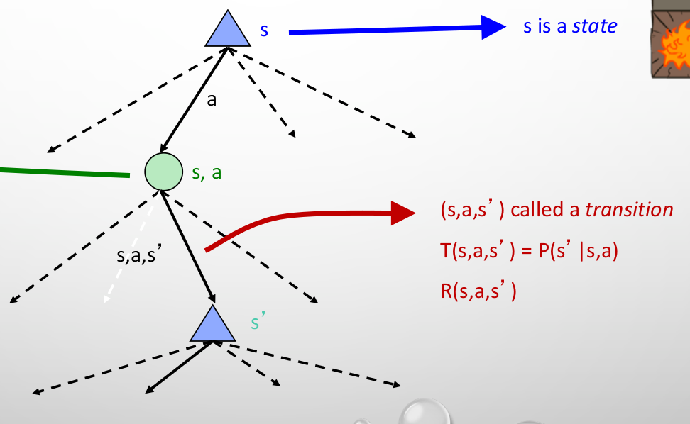
Set of states (S)

A set of actions (A)

Transition Function → T (s, a, s') -->This function takes the current state of s and gives the probability of going to the state of S 'by moving a. In other words, it gives p(s' | s, a).

Reward function R (s, a, s'), which gives us the reward of going from s to s' and can also be shown as R(s), R(s').

We have a start state

We may have a terminal state

Description Model

We have an environment, we give a as an input, then it takes us to the destination state and gives an output.

The Markov Property

In the Markov process, we assume that if we show the state at time t + 1 and look at it as a random variable and condition it based on what the state and action were in the previous moments (evidence), Then the state at the moment t + 1 depends only on the state at the moment t and the action at the moment t. This means that if we know the present state, the past and the future of that state are independent. The transfer function T shows the same information.

$$ P(S_{t+1} =s'| S_t = s_t, A_t=a_t, ...S_0 = s_0) $$

$$ = $$

$$ P(S_{t+1} =s'| S_t = s_t, A_t=a_t) $$

Policies

If our agent is in a deterministic environment, the goal is to find an optimal plan that responds to us. In an uncertain environment, instead of wanting for a complete plan, we look for a policy that takes one state as input and selects the next state accordingly.

so instead of returning a sequence, a function is given that is valid for all modes. A policy is good if it maximizes the average rewards

The policy method is like expectimax which the results are indefinite, the difference is that expectimax does not give us the policy and the tree has to be dragged and in any case there is no specific action.

On the other hand,without complete tree being calculated, the result can not be decided so expectimax method is time-consuming and in practice, the policy is used.

Sample Review

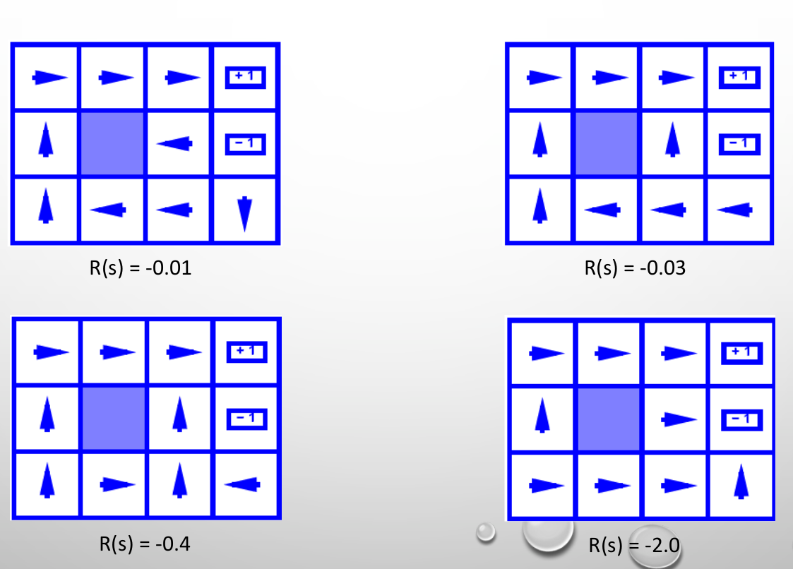R (s) = - 0.01

In this form, we go around to the answer that the hard way has been chosen to not have a negative penalty of one at all. This method, although it has a good average reward, but it is time consuming and will have a high repetition movement.

R (s) = - 0.03

A move to the wall has been replaced, which, although we are still far away, is done once and is faster, but has a lower reward overall.

R (s) = - 0.04

In this form, we are no longer far and the closest way has been chosen.

R (s) = - 2

Because the cost of travel is very high, the closest route is chosen from each house, regardless of the penalty.

Racing Example

Description

Consider a car that is racing and can have three states. The goal is to find the best way for a long trip in the fastest time possible. Reward 1 has been selected for slow movement and rewards 2 for fast movement. moving fast in warm state with a probability of one and fine of -10 will end up in overheated state.

Racing Search Tree

In this method, we first try to draw Expectimax.

MDP Search Tree

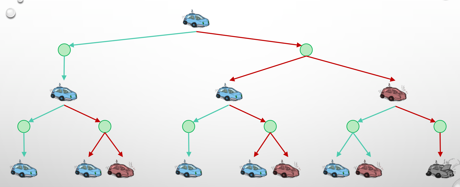
Each state is connected to the next states with probabilities and forms a tree. The difference between this tree and the expectimax tree is that we have rewards on each edge, but in expectimax we get rewards at the end, and the similarity in choosing an action with more rewards at each state.

Utilities of Sequences

This method requires a collective function that gives us the sum of rewards at each state until we reach the goal. This function must distinguish between two methods, receiving each reward in one state and summing all the rewards in the last state.

Preferences

Select more values

At each state,when there is two different action sequence with length of k which result the same value, we choose the early reward rather than late reward.

Discounting

Discounting makes coefficients for each state reward, which in the current case considers the coefficient 1, in the next case the coefficient Y, and in the third case, the coefficient $ Y ^ 2 $, and in this way calculates the sum of the rewards in each stage.

Quiz: Discounting

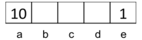For y = 1:

Because we are in d, it is better to go to 10

For y = 0.1:

It is better to go from d to 1 because if we go to 10, we will get a reward of 0.1.

For the same result: You solve the equation $10y ^ 2 = 1$

Reasons for the Reward Method

Stationary Preference

To some extent the behavior is the same and from one state to another we have the same sequence. We have the same comparison and we have a pattern that gives us the same behavior over time.

if we assume stationary preferences:

$ [a_1,a_2,...] > [b_1,b_2,...] $ $ <=> $ $ [r,a_1,a_2,...] > [r,b_1,b_2,...] $

there are two ways to define utilities:

Additive utility: $ U([r_0,r_1,...]) = r_0 + r_1 + ...$

Discounted utility: $ U([r_0,r_1,...]) = r_0 + yr_1 + y^2r_2 + ...$

Infinite Utility

use $ 0<\gamma<1 $

$$ U([r_0,...r_\infty]) = \sum_{t=0}^{\infty} \gamma^tr_t <= R_max/(1-\gamma) $$

If the program lasts indefinitely, the rewards can normally be infinite, and gamma and the discounting method can be used to achieve the following relationship using gamma, which limits the amount of rewards.

Optimal Quantities

V * (s): Average reward function provided optimal policy

Q * (s): Starting with the desired s and action and then performing the optimal operation

$$ V^*(s) = max_aQ^*(s,a) $$

$$ Q^*(s,a) = \sum_{s'}T(s,a,s') [R(s,a,s') + \gamma V^*(s')] $$

Recursive definition of value:

$$ V^*(s) = max_a\sum_{s'}T(s,a,s') [R(s,a,s') + \gamma V^*(s')] $$

Formal Definition of MDPs

Formally, a Markov decision process is defined by a tuple (S, $S_{0}$ ,A, T ,R,γ), where:

1. S is the state space, which contains all possible states the system may be in
2. $S_{0}$ is the start state
3. A is the action space, which contains all possible actions the agent may take when interacting with the system.
4. T : S × A → S′ is the transition dynamics. For each state s and action a, T(s, a) yields a probability distribution over states that the system may transition into when taking action a from state s. We sometimes write the conditional density/mass of transitioning into state s′ as P(s′ | s, a).
5. R : S ×A×S → R is the reward function. The value R(s, a, s′) gives the amount of “reward” associated transitioning into state s′ when taking action a from state s.
6. γ ∈ [0, 1] is the discount factor, which determines how much future rewards should be “discounted” when making decisions. A value of γ = 0 means that we don’t care about future rewards at all, while a value of γ = 1 indicates that rewards in the distant future should count just as much as the reward at the next time-step.

A policy π determines what action(s) to take at each state. 2 A stochastic policy π : S → ∆(A) assigns a distribution over actions to each state. Utility which we wish to maximize is sum of discounted rewards.

Value Functions

It is often useful to estimate how “good” a given state (and action) is. The standard tools for this are the Q-function (which considers a given state and action) and the value function (which considers a state only). These are defined:

$Q^{\pi}(s,a) := {\bf E}^{\pi}\Big[ \sum \limits _{t=1} ^{\infty} \gamma^{t} R_{t}|s_{0}=s ,a_{0}=a \Big]$

$V^{\pi}(s,a) := {\bf E}^{\pi}\Big[ \sum \limits _{t=1} ^{\infty} \gamma^{t} R_{t}|s_{0}=s \Big]$

now lets test the deffinition in an example:

aleread defined in previous chapters

Optimal Value Functions

Optimal value functions are best achievable expected returns (?). The optimal policy maximizes value function over all policies:

$Q^{*}(s,a) =max_{\pi}Q^{\pi}(s,a)$

$V^{*}(s) =max_{\pi}V^{\pi}(s)$

our main goal is finding $Q^{*}(s,a)$ and $V^{*}(s) $ for all states

Bellman Equations and Operators

Combining previously shown relationships between the value functions, we can derive the following recurrences, known as Bellman equations (after Richard Bellman):

$Q^{\pi}(s,a)={\bf E}_{S'} \Big[R(s,a,s') +{\gamma}{\bf E}_{a'} Q^{\pi}(s',a') \Big]$

$Q^{*}(s,a)={\bf E}_{S'} \Big[R(s,a,s') +{\gamma}max_{a'} Q^{*}(s',a') \Big]$

$V^{\pi}(s)={\bf E}_{a} \Big[{\bf E}_{s'} [R(s,a,s') +{\gamma}V^{\pi}(s')] \Big]$

$V^{*}(s)=max_{a} \Big[{\bf E}_{s'}[R(s,a,s') +{\gamma}V^{*}(s') ]\Big]$

Or, without the expectation operator:

$V^{\pi}(s)=max_{a}\Sigma_{s'} {T(s,a,s')} \Big [R(s,a,s') +{\gamma}V^{*}(s') \Big]$

This is a set of linear equations one for each state.The value function for π is its unique solution

An optimal policy can be found by maximizing over $Q^{*}(s,a)$. i.e. Find sequence of actions from current state to goal , that maximizes utility We know how to do this using earlier search techniques In the maze example, $\pi$(s) associates a motion to a particular location on the grid For any state s, the utility is the sum of discounted rewards of the sequence of states starting at sgenerated by using the policy $\pi$

Value Iteration

Racing tree drawbacks

1. We’re doing way too much work
2. States are repeated and we must Only compute needed quantities once 3.another Problem is that the Tree goes on forever.

our idea is Doing a depth-limited computation, but with increasing depths until change is small ( deep parts of the tree eventually don’t matter if γ < 1)

One way, to find an optimal policy is to find the optimal value function. It can be determined by a simple iterative algorithm called value iteration that can be shown to converge to the correct $V^{*}$ values

We are going to compute $V(s)$ for all s, by doing an iterative procedure, in which our current estimate for $V^{*}(s)$ gets closer to the true value over time. We start by initializing $V^{*}(s)$ to 0, for all states. We could actually initialize to any values we wanted to, but it’s easiest to just start at 0. Now, we loop for a while Let’s say we want to guarantee that when we terminate, the current value function differs from $V^{*}$ by at most assumed epsilon.

Loop for all s $V_{K+1}(s) \leftarrow max_{a}\Sigma_{s'} {T(s,a,s')} \Big [R(s,a,s') +{\gamma}V_{k}(s') \Big]$ In order to guarantee this condition, it is sufficient to examine the maximum difference between Vt and Vt+1.

Now, although we may never converge to the exact, analytically correct V* in a finite number of iterations, it’s guaranteed that we can get close enough to V* so that using V to choose our actions will yield the optimal policy within a finite number of iterations. In fact, using value iteration, we can find the optimal policy in time that is polynomial in the size of the state and action spaces, the magnitude of the largest reward$(O(S^{2}A))$

Policy Iteration

The previously discussed algorithms aim to approximate the optimal value functions directly. Policy iteration is a different approach based on two alternating steps:

1. Policy evaluation: compute $Q^{\pi_{k}}$ , the value of the current policy $\pi_{k}$

$V_{K+1}^{\pi_{i}}(s) \leftarrow max_{a}\Sigma_{s'} {T(s,\pi_{i}(s),s')} \Big [R(s,\pi_{i}(s),s') +{\gamma}V^{\pi_{i}}_{k}(s') \Big] \quad \quad \quad \quad (1)$

2. Policy improvement: update the policy as $\pi_{k+1}$=$\pi_{Q^{\pi_{k}}}$ , the greedy policy with respect to the Q function of the previous policy

${\pi}_{i+1}(s)=max_{a}\Sigma_{s'} {T(s,a,s')} \Big [R(s,a,s') +{\gamma}V^{\pi_{i}}(s') \Big] \quad \quad \quad \quad \quad \quad \quad \quad (2)$

Note that each policy evaluation, itself an iterative computation, is started with the value function for the previous policy. This typically results in a great increase in the speed of convergence of policy evaluation (presumably because the value function changes little from one policy to the next). The policy improvement theorem assures us that these policies are better than the original random policy. In this case, however, these policies are not just better, but optimal, proceeding to the terminal states in the minimum number of steps.

The policy iteration algorithm is based on the observation that we can also view in above Equation. Notice that the left hand side, ${\pi}_{i+1}$ appears on the right hand side.This is precisely the shape of a fixed point equation. This observation suggests that we can use a similar procedure to value iteration: we begin with any policy ${\pi}_{0}$, apply the right hand side of equation 2 to generate a new policy ${\pi}_{1}$, apply the right hand side again to get ${\pi}_{2}$, and so on. The process is a little more complicated than for value iteration. In value iteration, applying the right hand side of Equation to any previous value function $V$ is easy. For policy iteration, it is not quite as straightforward to apply the right hand side of equation 2 to a policy ${\pi}$.we need to evaluate equation 1 with current policy to aquire maximum value function for this state. so this action is cnosist of two acts: for a fixed policy, the value function $v_{\pi}$ satisfies equation 1 . So, given ${\pi}$, we solve Equations , which is a system of linear equations, to obtain $v_{\pi}$. We then apply the right hand side of equation 2 to get a new policy. That is, we do a step of policy evaluation and then a step of policy improvement.
Note that we repeat until the policy stops changing. Policy iteration is a neat idea.

Proof of Convergence property of policy iteration involves showing that each iteration is also a contraction, and policy must improve each step, or be optimal policy

Interesting theoretical note is that ,since number of policies is finite (though exponentially large), policy iteration converges to exact optimal policy

you can read Convergence Proofs for Value and PolicyIteration with more detail here https://arxiv.org/pdf/2009.11403.pdf

Comparing Value Iteration and Policy Iteration

How do value iteration and policy iteration compare? It is a fact that policy iteration takes at most as many iterations to reach the optimal policy as value iteration does. In practice, it usually takes far fewer iterations.each individual iteration of policy iteration takes longer, because it requires solving the complete system of linear equations . This can be done via Gaussian elimination, for example, in $o(n^{3})$ Compared to value iteration, in which each step of the algorithm takes $o(NML)$ (for NM updates of Q-values, on N states and M actions, with each taking time L where L is the max number of states reachable by any action a from any state s.) In general, however, policy iteration is considered the better algorithm in practice.

CONCLUSION:

In value iteration:

• Every iteration updates both the values and (implicitly) the policy
• We don’t track the policy, but taking the max over actions implicitly recomputes it

In policy iteration:

• We do several passes that update utilities with fixed policy (each pass is fast because we consider only one action, not all of them)
• After the policy is evaluated, a new policy is chosen (slow like a value iteration pass)
• The new policy will be better (or we’re done)