
matinamehdizadeh
Author
In this notebook, we introduce recurrent neural networks and the sequence modeling ideas behind them.
Traditional feed-forward neural networks take in a fixed amount of input data all at the same time and produce a fixed amount of output each time. However, in some context in machine learning we want to have more flexibility in the types of data that our model can process. therefore, we move to this idea of recurrent neural networks (RNN). A recurrent neural network is a special type of an artificial neural network adapted to work for time series data or data that involves sequences; Meaning, RNNs do not consume all the input data at once. Instead, they take them in one at a time and in a sequence. At each step, the RNN does a series of calculations before producing an output. The output, known as the hidden state, is then combined with the next input in the sequence to produce another output. This process continues until the model is programmed to finish or the input sequence ends. To sum up, RNNs have the concept of memory that helps them store the states or information of previous inputs to generate the next output of the sequence.

We can think about RNNs in two ways. one is this concept of having a hidden state that feeds back at itself recurrently. The other one is to think about unrolling this computational graph for multiple time steps. This would help understanding the recurrent network easier.

$x_t$ is the input at time step t. To keep things simple we assume that $x_t$ is a scalar value with a single feature. You can extend this idea to a d-dimensional feature vector. $o_t$ is the output of the network at time step t. We can produce multiple outputs in the network but for this example we assume that there is one output. $h_t$ vector stores the values of the hidden states at time t. This is also called the current context. $h_0$ vector is initialized to zero. $w_t$ is weight matrix. At every time step we can unfold the network for k time steps to get the output at time step k+1. The unfolded network is very similar to the feedforward neural network. Now that we are seeing recurrent neural network as an feedforward neural network with k step, we can easily compute the outputs.
During training, for each piece of training data we will have a corresponding ground-truth label that we want the model to output. After receiving these outputs, we will calculate the loss of that process, which measures how far off, the model’s output is from the correct answer. Using this loss, we can calculate the gradient of the loss function for back-propagation. With the gradient that we just obtained, we can update the weights in the model accordingly. Combined with the forward pass, back-propagation is looped over and again, allowing the model to become more accurate with its outputs each time as the weight matrices values are modified to pick out the patterns of the data.
Although it may look as if each RNN cell is using a different weight as shown in the graphics, all of the weights are actually the same as that RNN cell is essentially being re-used throughout the process. This may lead to one of RNNs disadvantages which is the vanishing gradient problem, where the gradients used to compute the weight update may get very close to zero due to multiplication of the same matrix over and over again which prevents the network from learning new weights. The deeper the network, the more pronounced is this problem.
The pseudo-code for training is given below. The value of k which is the recursion factor can be selected by the user for training. In the pseudo-code below $p_t$ is the target value at time step t:
Repeat till stopping criterion is met: Set all h to zero. Repeat for t = 0 to k Forward propagate the network over the unfolded network for k time steps to compute all h and y. Compute the error as: $error = y_{k} - p_{k}$ Backpropagate the error across the unfolded network and update the weights.
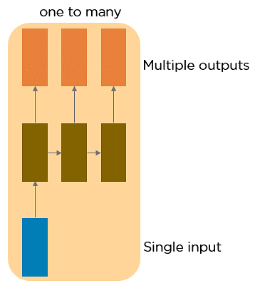
RNNs are really flexible and can adapt to your needs. As you will see in the images below, your input and output size can come in different forms, yet they can still be fed and extracted from the RNN model. There are different types of recurrent neural networks with varying architectures that are shown below.
This type of neural network has a input which is an object of fixed size like an image and the output is a sequence of variable lenght, such as a caption where diffrent captions might have diffrent number of words, so our output needs to be variable at lenght.
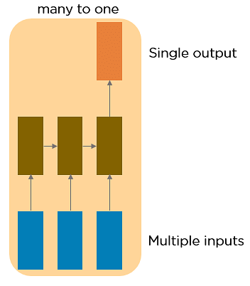
This RNN takes a sequence of inputs that could be variably sized like a text and generates a single output. Sentiment analysis is a good example of this kind of network where a given sentence can be classified as expressing positive or negative sentiments or in a computer vision contex, you might imagine taking as input, a video which might have variable number of frames and we want to read this entire video of potentioally variable lenght and at the end, make a classification decision about the kind of activity that is going on in that video.
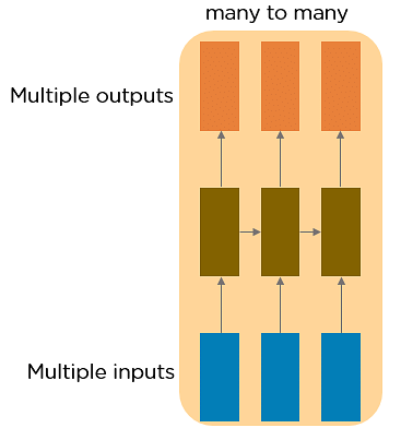
This RNN takes a sequence of inputs and generates a sequence of outputs. Machine translation is one of the examples where our input might be some sentence in English, which could have a variable lenght and our output is the same sentence but in French, which also could have a variable length and crucially the length of the English sentence might be diffrent from the lenght of the French sentence so we need some models that have the capacity to accept both variable length sequences on the input and the output.
We might also consider problems in computer vision contex, where our input is variably length like a video sequence with variable number of frames and we want to make a decision for each element of that input sequence. which in the context of video, is making a classification decision along every frame of that video.
As we saw above, RNNs are like a general paradigm for handling variable sized sequenced data that allow us to capture all of these diffrent types of setups in our models.
In this example we will be implementing a simple RNN character model with PyTorch to familiarize ourselves with the PyTorch library and get started with RNNs. In this implementation, we will be building a model that can complete your sentence based on a few characters or a word used as input.
We will start off by installing and importing the main packages that we will use.
#!pip3 install torch
# !pip3 install numpy
import torch
from torch import nn
import numpy as np
We have to set our device first. we would use gpu if available and cpu if not.
if torch.cuda.is_available():
    device = torch.device("cuda")
    print("GPU is available")
else:
    device = torch.device("cpu")
    print("GPU not available, CPU used")
GPU not available, CPU used
Then, we will define the sentences that we want our model to output when fed with the first word or the first few characters and create a dictionary out of all the characters that we have in the sentences and map them to an integer.
text = ['hey how are you','good i am fine','have a nice day']
chars = set(''.join(text))
int2char = dict(enumerate(chars))
char2int = {char: ind for ind, char in int2char.items()}
Next, we will be padding our input sentences to ensure that all the sentences are of the sample length. While RNNs are typically able to take in variably sized inputs, we will usually want to feed training data in batches to speed up the training process. In order to used batches to train on our data, we'll need to ensure that each sequence within the input data are of equal size.
Therefore, in most cases, padding can be done by filling up sequences that are too short with 0 values and trimming sequences that are too long. In our case, we'll be finding the length of the longest sequence and padding the rest of the sentences with blank spaces to match that length.
maxlen = len(max(text, key=len))

for i in range(len(text)):
    while len(text[i])<maxlen:
        text[i] += ' '
As we are going to predict the next character in the sequence at each time step, we will have to divide each sentence into Input data and Target. Also, we should be careful that the last input character should be excluded as it does not need to be fed into the model.
Our target is one time-step ahead of the Input data as this will be the answer for the model at each time step corresponding to the input data.
At the end we convert our input and target sequences to sequences of integers instead of characters by mapping them using the dictionaries we created before. This will allow us to one-hot-encode our input sequence subsequently.
input_seq = []
target_seq = []

for i in range(len(text)):
    input_seq.append(text[i][:-1])
    target_seq.append(text[i][1:])
    print("Input Sequence: {}\nTarget Sequence: {}".format(input_seq[i], target_seq[i]))

for i in range(len(text)):
    input_seq[i] = [char2int[character] for character in input_seq[i]]
    target_seq[i] = [char2int[character] for character in target_seq[i]]
Input Sequence: hey how are yo
Target Sequence: ey how are you
Input Sequence: good i am fine
Target Sequence: ood i am fine
Input Sequence: have a nice da
Target Sequence: ave a nice day
Then we encode our input sequence into one-hot vectors and convert them to tensors.
dict_size = len(char2int)
seq_len = maxlen - 1
batch_size = len(text)

def one_hot_encode(sequence, dict_size, seq_len, batch_size):
    features = np.zeros((batch_size, seq_len, dict_size), dtype=np.float32)

    for i in range(batch_size):
        for u in range(seq_len):
            features[i, u, sequence[i][u]] = 1
    return features

input_seq = one_hot_encode(input_seq, dict_size, seq_len, batch_size)
print("Input shape: {} --> (Batch Size, Sequence Length, One-Hot Encoding Size)".format(input_seq.shape))

input_seq = torch.from_numpy(input_seq)
target_seq = torch.Tensor(target_seq)
Input shape: (3, 14, 17) --> (Batch Size, Sequence Length, One-Hot Encoding Size)
To start building our own neural network model, we can define a class that inherits PyTorch’s base class (nn.module) for all neural network modules. After doing so, we can start defining some variables and also the layers for our model under the constructor. For this model, we wll only be using one layer of RNN followed by a fully connected layer. The fully connected layer will be in-charge of converting the RNN output to our desired output shape.
We also have to define the forward pass function under forward() as a class method. The order the forward function is sequentially executed, therefore have to pass the inputs and the zero-initialized hidden state through the RNN layer first, before passing the RNN outputs to the fully-connected layer.
The last method that we have to define is the method that we called earlier to initialize the hidden state - init_hidden(). This basically creates a tensor of zeros in the shape of our hidden states.
Then we create an instance of our model and initialize the hyperparameters and start the training process.
class Model(nn.Module):
    def __init__(self, input_size, output_size, hidden_dim, n_layers):
        super(Model, self).__init__()

        self.hidden_dim = hidden_dim
        self.n_layers = n_layers
        self.rnn = nn.RNN(input_size, hidden_dim, n_layers, batch_first=True)
        self.fc = nn.Linear(hidden_dim, output_size)

    def forward(self, x):

        batch_size = x.size(0)
        hidden = self.init_hidden(batch_size)
        out, hidden = self.rnn(x, hidden)
        out = out.contiguous().view(-1, self.hidden_dim)
        out = self.fc(out)

        return out, hidden

    def init_hidden(self, batch_size):
        hidden = torch.zeros(self.n_layers, batch_size, self.hidden_dim).to(device)
        return hidden
model = Model(input_size=dict_size, output_size=dict_size, hidden_dim=12, n_layers=1)
model = model.to(device)

n_epochs = 100
lr=0.01

criterion = nn.CrossEntropyLoss()
optimizer = torch.optim.Adam(model.parameters(), lr=lr)
input_seq = input_seq.to(device)
for epoch in range(1, n_epochs + 1):
    optimizer.zero_grad() # Clears existing gradients from previous epoch
    #input_seq = input_seq.to(device)
    output, hidden = model(input_seq)
    output = output.to(device)
    target_seq = target_seq.to(device)
    loss = criterion(output, target_seq.view(-1).long())
    loss.backward() # Does backpropagation and calculates gradients
    optimizer.step() # Updates the weights accordingly

    if epoch%10 == 0:
        print('Epoch: {}/{}.............'.format(epoch, n_epochs), end=' ')
        print("Loss: {:.4f}".format(loss.item()))
Epoch: 10/100............. Loss: 2.5228
Epoch: 20/100............. Loss: 2.1118
Epoch: 30/100............. Loss: 1.7116
Epoch: 40/100............. Loss: 1.3229
Epoch: 50/100............. Loss: 0.9832
Epoch: 60/100............. Loss: 0.7112
Epoch: 70/100............. Loss: 0.5081
Epoch: 80/100............. Loss: 0.3617
Epoch: 90/100............. Loss: 0.2649
Epoch: 100/100............. Loss: 0.2016
Now we have to test our model.
def predict(model, character):
    character = np.array([[char2int[c] for c in character]])
    character = one_hot_encode(character, dict_size, character.shape[1], 1)
    character = torch.from_numpy(character)
    character = character.to(device)

    out, hidden = model(character)

    prob = nn.functional.softmax(out[-1], dim=0).data
    char_ind = torch.max(prob, dim=0)[1].item()

    return int2char[char_ind], hidden
def sample(model, out_len, start='hey'):
    model.eval()
    start = start.lower()
    chars = [ch for ch in start]
    size = out_len - len(chars)
    for ii in range(size):
        char, h = predict(model, chars)
        chars.append(char)

    return ''.join(chars)
sample(model, 15, 'good')
'good i am fine '
As we can see, the model is able to come up with the sentence ‘good i am fine ‘ if we feed it with the words ‘good’, achieving what we intended for it to do.
In this notebook we discuss:
This is just the tip of the iceberg when it comes to Recurrent Neural Networks. While the vanilla RNN is rarely used in solving NLP or sequential problems, having a good grasp of the basic concepts of RNNs will definitely aid in your understanding as you move towards the more popular GRUs and LSTMs.
Recurrent Neural Networks Lecture, Stanford University School of Engineering Recurrent Neural Network (RNN) Tutorial: Types, Examples, LSTM and More RNN walkthrough An Introduction To Recurrent Neural Networks And The Math That Powers Them A Tour of Recurrent Neural Network Algorithms for Deep Learning A Beginner’s Guide on Recurrent Neural Networks with PyTorch